8 Chapters 7 and 8 problems
- Baumann and Jones of the Purdue University Education Department conducted an experiment to compare different methods for reaching reading comprehension in children. Three methods were compared, but here we will consider two only:
- Basal - using textbooks designed to develop reading skills
- Directed Reading Thinking Activity (DRTA) - a comprehension strategy that guides students in asking questions about a text, making predictions, and then reading to confirm or refute their predictions.
Twenty-two children were randomly allocated to each of these methods (so that we might expect similar abilities between the two groups at the start), and their reading comprehension was tested before and after instruction. Here, we just analyse scores after instruction. Histograms of the data are shown in the next plot.

Figure 8.1: Histograms of reading comprehension scores for children taught by the basal and DRTA methods. From the data, we want to determine which method is best on average.
The scores are stored in the R vectors basal and drta. Some R output is given below.
basal## [1] 5 9 5 8 10 9 12 5 8 7 12 4 4 8 6 9 3 5 4 2 5 7drta## [1] 7 5 13 5 14 14 10 13 12 11 8 7 10 8 8 10 12 10 11 7 8 12c(mean(basal), var(basal), mean(drta), var(drta))## [1] 6.682 7.656 9.773 7.422- Write down a suitable model for the data, defining your notation carefully. You can assume test scores are normally distributed.
- State appropriate null and alternative hypotheses, in terms of your model parameters, to test whether the mean scores are different between the two methods.
- For an appropriate two-sample \(t\)-test, calculate the value of the test statistic
- Draw a sketch to illustrate what the \(p\)-value would represent, indicating the value of your test statistic.
- Give the R command needed to find the \(p\)-value.
- How would you interpret a \(p\)-value less than 0.001, with reference to the two teaching methods?
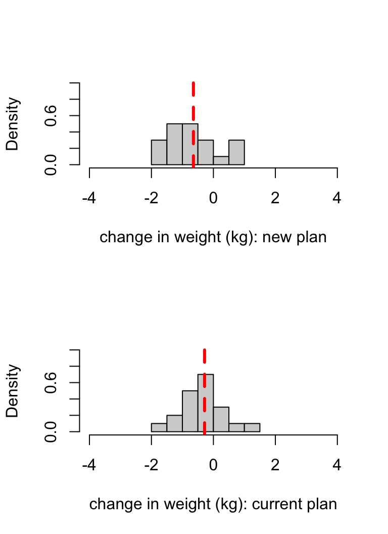
- A new 12 week weight-loss plan has been designed to help adults with a body mass index (BMI) \(>\) 25 lose weight. Forty volunteers are recruited to a study to test the plan. Half the volunteers are assigned to the new plan, and the other half are assigned to an alternative plan: one that is currently recommended. The change in weight (in kg) is measured for each adult at the end of the study. The interest is in whether the new plan is any more effective than the current one.
- Assume the changes in weight in the two groups are normally distributed. Defining your notation carefully, write down a null and alternative hypotheses that would be appropriate for testing whether the new plan is more or less effective than the current one.
- Histograms for the two groups are shown below. The sample mean is indicated by the dashed line in each case. Note that the sample mean was lower (more weight lost on average) in the group with the new plan. If your hypothesis test in part (a) was to be conducted, at the 5% level of significance (so that you are using the Neyman-Pearson framework), by studying the plot below, what do you think the result would be? Briefly explain your answer.
- The changes in weight for the two groups are stored in R as the vectors
newplanandcurrentplanrespectively. Using the following R output, test your hypothesis in part a at the 5% level of significance. Assume that for \(\nu >30\), you can approximate the \(t_\nu\) distribution by the \(N(0,1)\) distribution. State clearly the conclusion of your test, in terms of whether there is evidence from the experiment that the new plan is more effective than the current plan.
c(mean(newplan), var(newplan))## [1] -0.6450 0.7089c(mean(currentplan), var(currentplan))## [1] -0.285 0.515qnorm(0.975)## [1] 1.96- Using (some of) the following R output, deduce an interval within which the \(p\)-value from your hypothesis test must lie.
qnorm(c(0.9, 0.95, 0.975))## [1] 1.282 1.645 1.960- Calculate a 95% confidence interval for the difference between the two population means, again, assuming that for \(\nu >30\), you can approximate the \(t_\nu\) distribution by the \(N(0,1)\) distribution. By inspecting your interval, what would be the outcome of a test of the null hypothesis, of size 0.05, that patients on the new plan lose, on average 0.5kg more than patients on the current plan? Would this contradict your earlier conclusion?
- Two driving instructors are to be compared regarding how many of their pupils pass their driving tests at the first attempt. Instructor A has 30 pupils, and 18 pass at the first attempt. Instructor B has 35 pupils, and 12 pass at the first attempt. Conduct a suitable hypothesis to compare the two instructors.
- State your model for the data and define your notation carefully.
- Draw a sketch to indicate your observed test statistic and \(p\)-value.
- State the R command you would use to get the \(p\)-value.
- How would a \(p\)-value of 0.04 be interpreted in this case?
- Suppose we have two binomial random variables \[\begin{align*} X&\sim Bin(n, \theta_X),\\ Y&\sim Bin(m, \theta_Y), \end{align*}\] and we wish to test the null hypothesis \[ H_0: \theta_X = \theta_Y. \] We use the test statistic \[ Z:= \frac{\frac{X}{n} - \frac{Y}{m}}{\sqrt{v}} \] where \[ v:= p^*(1-p^*)\left(\frac{1}{n} + \frac{1}{m}\right), \] and \[ p^*: = \frac{x+y}{n+m}. \] If we assume \(H_0\) is true, and we further assume \(\theta_X = \theta_Y = \frac{x+y}{n+m}\), then prove that
\[\begin{align} \mathbb{E}(Z) &= 0,\\ Var(Z)&=1. \end{align}\]
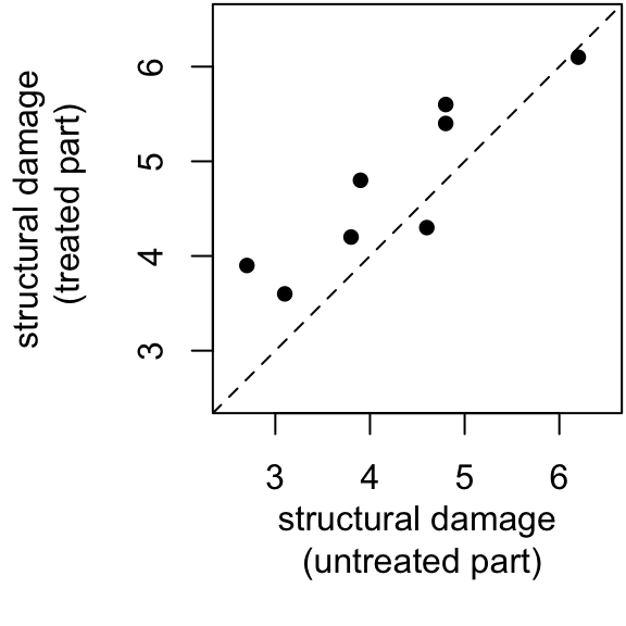
- Challenge problem. In an investigation into the effects of a pesticide on the leaves of a plant, eight leaves were chosen and each was divided into two parts. One part of each leaf was treated with the pesticide and the other was not. Microscopic examination of the leaves for structural damage gave the following comparative responses, where a higher number corresponds to more damage. A scatter plot of these data are shown below. The dashed line has gradient 1 and \(y\)-intercept 0.
Suppose the observations are normally distributed, and consider the following R output
untreated <- c(2.7, 4.6, 3.8, 4.8, 3.9, 6.2, 4.8, 3.1)
treated <- c(3.9, 4.3, 4.2, 5.4, 4.8, 6.1, 5.6, 3.6)
differences <- untreated - treated
t.test(untreated, treated)
##
## Welch Two Sample t-test
##
## data: untreated and treated
## t = -1, df = 13, p-value = 0.3
## alternative hypothesis: true difference in means is not equal to 0
## 95 percent confidence interval:
## -1.5809 0.5809
## sample estimates:
## mean of x mean of y
## 4.237 4.737t.test(differences)##
## One Sample t-test
##
## data: differences
## t = -2.8, df = 7, p-value = 0.03
## alternative hypothesis: true mean is not equal to 0
## 95 percent confidence interval:
## -0.9192 -0.0808
## sample estimates:
## mean of x
## -0.5In the second \(t\)-test, a one-sample \(t\)-test has been conducted. For a one-sample \(t\) test, we have random variables \[ X_1,\ldots,X_n\stackrel{i.i.d}{\sim}N(\mu, \sigma^2), \] we test the hypothesis \(H_0:\mu = 0\), and our test statistic is \[ T = \frac{\bar{X}}{\sqrt{S^2/n}}\sim t_{n-1}, \] assuming \(H_0\) is true.
Do the two \(p\)-values give contradictory conclusions? If not, why not?