Chapter 7 Parameter estimation
In this Chapter we study how to fit a linear model to some observed data, i.e., how to use the data to estimate the model parameters. Recall the disputed election example (re-plotted below, with the contested election omitted).
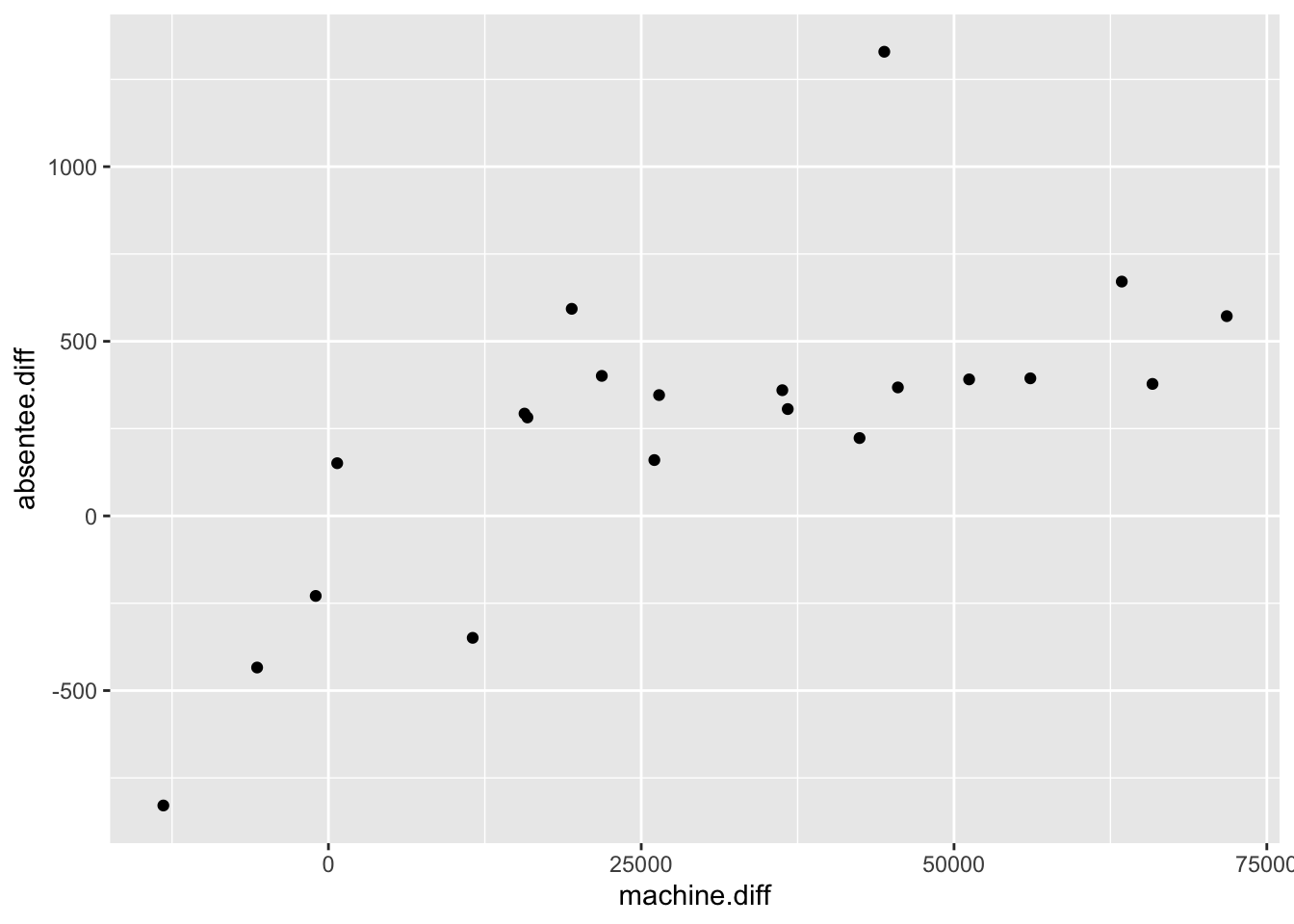
Figure 7.1: Difference in absentee votes (Democrat - Republican) against difference in machine votes (Democrat - Republican) against in 21 different elections in Philadelphia’s senatorial districts.
For election \(i\) let \(x_i\) denote the difference in machine votes (Democrat \(-\) Republican) and \(y_i\) denote the observed difference in absentee votes (Democrat \(-\) Republican). We’ll consider the simple linear regression model, and in a slight abuse of notation we will write \[\begin{equation} y_i=\beta_0 + \beta_1 x_i + \varepsilon_i, \end{equation}\] for \(i=1,\ldots,n\). (Because \(y_i\) is an observed value rather than a random variable \(Y_i\), the error term \(\varepsilon_i\) is now a constant: the ‘realised’ error rather than a random variable with the \(N(0,\sigma^2)\) distribution. But we will not make this distinction in our notation.)
The unknown parameters to be estimated are \(\beta_0,\beta_1\) and \(\sigma^2\). We will consider how to estimate \(\beta_0\) and \(\beta_1\) first and deal with \(\sigma^2\) later.
7.1 Least squares estimation
Firstly, we rearrange the above equation to get \[ \varepsilon_i=y_i - \beta_0 - \beta_1 x_i. \] Since we know the values of \(y_i\) and \(x_i\), for any choice of \((\beta_0,\beta_1)\) we can then calculate the implied values of \(\varepsilon_i\). Note that in this model the random error term has expectation 0, and so small (absolute) values of the errors are more probable than large (absolute) values. Additionally, some choices of \((\beta_0,\beta_1)\) are clearly better than others. Consider the following figure:
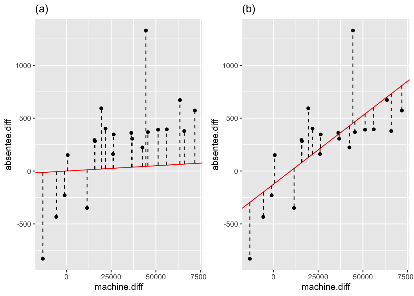
Figure 7.2: The solid line is \(y=\beta_0+\beta_1 x\), with \((\beta_0=0,\beta_1=0.001)\) in panel (a), and \((\beta_0=-125,\beta_1=0.013)\) in panel (b). Lengths of the dotted lines indicate the magnitude of each \(\varepsilon_i\).
We see that choosing \((\beta_0=-125,\beta_1=0.013)\) appears to fit the data better than choosing \((\beta_0=0,\beta_1=0.001)\) because the observed points lie closer to the line \(y=\beta_0 +\beta_1 x\). Specifically, we prefer \((\beta_0=-125,\beta_1=0.013)\) because on average \(|\varepsilon_1|,\ldots,|\varepsilon_n|\) are smaller:
| \(\sum_{i=1}^n |\varepsilon_i|\) | \(\sum_{i=1}^n \varepsilon_i^2\) | |
|---|---|---|
| \((\beta_0=0,\beta_1=0.001)\) | 8410 | 4,704,524 |
| \((\beta_0=-125,\beta_1=0.013)\) | 5018 | 2,007,945 |
This suggests we should choose \((\beta_0,\beta_1)\) to make \(\sum_{i=1}^n \varepsilon_i^2\) as small as possible (note that minimising \(\sum_{i=1}^n \varepsilon_i^2\) is easier than minimising \(\sum_{i=1}^n |\varepsilon_i|\)). Define \[\begin{equation}R(\beta_0,\beta_1)=\sum_{i=1}^n \varepsilon_i^2 = \sum_{i=1}^n (y_i-\beta_0-\beta_1 x_i)^2. \end{equation}\] The least squares estimates of \(\beta_0\) and \(\beta_1\) are the values of \(\beta_0\) and \(\beta_1\) that minimise \(R(\beta_0,\beta_1)\). Now \[\begin{eqnarray} \frac{\partial R(\beta_0,\beta_1)}{\partial \beta_0}&=& -2\sum_{i=1}^n(y_i-\beta_0-\beta_1 x_i),\\ \frac{\partial R(\beta_0,\beta_1)}{\partial \beta_1}&=& -2\sum_{i=1}^nx_i(y_i-\beta_0-\beta_1 x_i). \end{eqnarray}\] Let \(\hat{\beta}_0\) and \(\hat{\beta}_1\) denote the least squares estimates of \(\beta_0\) and \(\beta_1\). Since (by definition) \(\hat{\beta}_0\) and \(\hat{\beta}_1\) minimise \(R(\beta_0,\beta_1)\), both partial derivative must equal 0 at \(\beta_0=\hat{\beta}_0\) and \(\beta_1=\hat{\beta}_1\), so \[\begin{eqnarray} 0&=& -\sum_{i=1}^n(y_i-\hat{\beta}_0-\hat{\beta}_1 x_i),\\ 0&=& -\sum_{i=1}^nx_i(y_i-\hat{\beta}_0-\hat{\beta}_1 x_i), \end{eqnarray}\] which we can re-write as \[\begin{eqnarray} n\hat{\beta}_0 +\hat{\beta}_1\sum_{i=1}^n x_i &=& \sum_{i=1}^n y_i,\\ \hat{\beta}_0\sum_{i=1}^n x_i +\hat{\beta}_1 \sum_{i=1}^n x_i^2 &=& \sum_{i=1}^n x_iy_i, \end{eqnarray}\] and these can be solved simultaneously to give \[\begin{eqnarray} \hat{\beta}_1&=&\frac{n \sum_{i=1}^n x_i y_i -\sum_{i=1}^n x_i \sum_{i=1}^n y_i}{n \sum_{i=1}^n x_i^2 -\left(\sum_{i=1}^n x_i \right)^2}, \\ \hat{\beta}_0&=&\bar{y} - \hat{\beta}_1\bar{x}. \end{eqnarray}\]
Although you won’t need to calculate these terms by hand, we will tidy up these expressions to get the formulae that you may see in textbooks.
Define \[\begin{eqnarray} s_{xy}&=&\sum_{i=1}^n (x_i-\bar{x})(y_i-\bar{y}),\\ s_{xx}&=&\sum_{i=1}^n (x_i-\bar{x})^2. \end{eqnarray}\] Note that \(\sum_{i=1}^n (x_i-\bar{x})=0\) and so \(\sum_{i=1}^n(x_i-\bar{x})\bar{y}=\bar{y}\sum_{i=1}^n(x_i-\bar{x})=0\). Hence \[\begin{equation} s_{xy}=\sum_{i=1}^n(x_i-\bar{x})y_i = \sum_{i=1}^n x_i y_i -\frac{\sum_{i=1}^n x_i\sum_{i=1}^n y_i}{n}. \end{equation}\] Also, \[\begin{equation} s_{xx}=\sum_{i=1}^n x_i^2 - \frac{\left(\sum_{i=1}^n x_i\right)^2}{n}, \end{equation}\] and so we can write \[\begin{equation} \boxed{\,\hat{\beta}_1=\frac{s_{xy}}{s_{xx}}\quad\hat{\beta}_0=\bar{y}-\hat{\beta}_1\bar{x}.}\label{abhat} \end{equation}\]
We will see how to fit linear models in R later on, but for now, for the election data we can do
x <- election$machine.diff
y <- election$absentee.diff
beta1Hat <- sum((x - mean(x)) * (y - mean(y)))/
  sum((x - mean(x))^2)
beta0Hat <- mean(y) - beta1Hat * mean(x)
c(beta0Hat, beta1Hat)
## [1] -125.90364382 0.01270346So we have \(\hat{\beta}_0=-125.9036\) and \(\hat{\beta}_1=0.0127\). The line \(y=-125.9036+0.0127x\). This gives a line very close to that in panel (b) in Figure 7.2.
Example 7.1 (Least squares estimation: weights example.)
Continuing from Example 6.1, suppose the observed weights are denoted by \(y_1, y_2, y_3\). Derive the least squares estimates of \(\theta_A\) and \(\theta_B\)
Solution
We define \[ R(\theta_A, \theta_B) := \sum_{i=1}^3 \varepsilon_i^2 = (y_1-\theta_A)^2 + (y_2-\theta_B)^2+(y_3-\theta_A -\theta_B)^2. \] Then the least squares estimates are the solutions of \[\begin{align*} \frac{\partial R(\theta_A, \theta_B)}{\partial \theta_A} = -2(y_1-\theta_A) -2(y_3 - \theta_A-\theta_B) = 0,\\ \frac{\partial R(\theta_A, \theta_B)}{\partial \theta_B} = -2(y_2-\theta_B) -2(y_3 - \theta_A-\theta_B) = 0. \end{align*}\]
After a little algebra to solve these two equations simultaneously, we get \[ \hat{\theta}_A = \frac{2y_1 -y_2 + y_3}{3}, \quad \hat{\theta}_B = \frac{2y_2 -y_1 + y_3}{3}. \]
7.2 Assumptions for least squares
Note that we have not made use of the assumption that the errors \(\varepsilon_i\) are normally distributed. If we look again at the function we chose to minimise \[ R(\beta_0,\beta_1)=\sum_{i=1}^n \varepsilon_i^2 = \sum_{i=1}^n (y_i-\beta_0-\beta_1 x_i)^2, \] we note that each error \(\varepsilon_i\) has equal weight in the sum; we are not trying to make some errors smaller than others. This relates back to the assumption that the errors have equal variance; this is an assumption we should try to check. There are analyses we might choose to do that rely on the normality assumption, but these will not be the main focus in this module.
There are actually two ways in which a single observation might be unduly influential:
- the error \(\varepsilon_i\) is an outlier;
- the independent variable \(x_i\) is an outlier.
Case (1) may be the result of non-constant variance of the errors. An example is shown below.
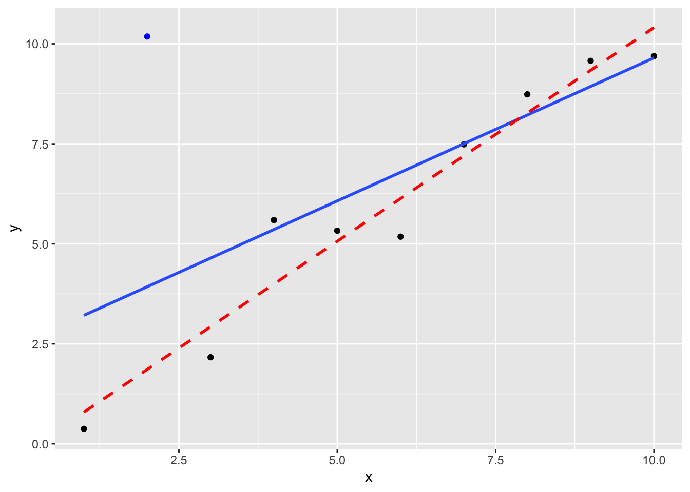
Figure 7.3: The blue line is the least squares fit using all ten observations. The red dashed line is the least squares fit, omitting the outlier (shown by the blue dot) at \(x=2\).
Case (2) is sometimes referred to as high leverage. We illustrate this below.
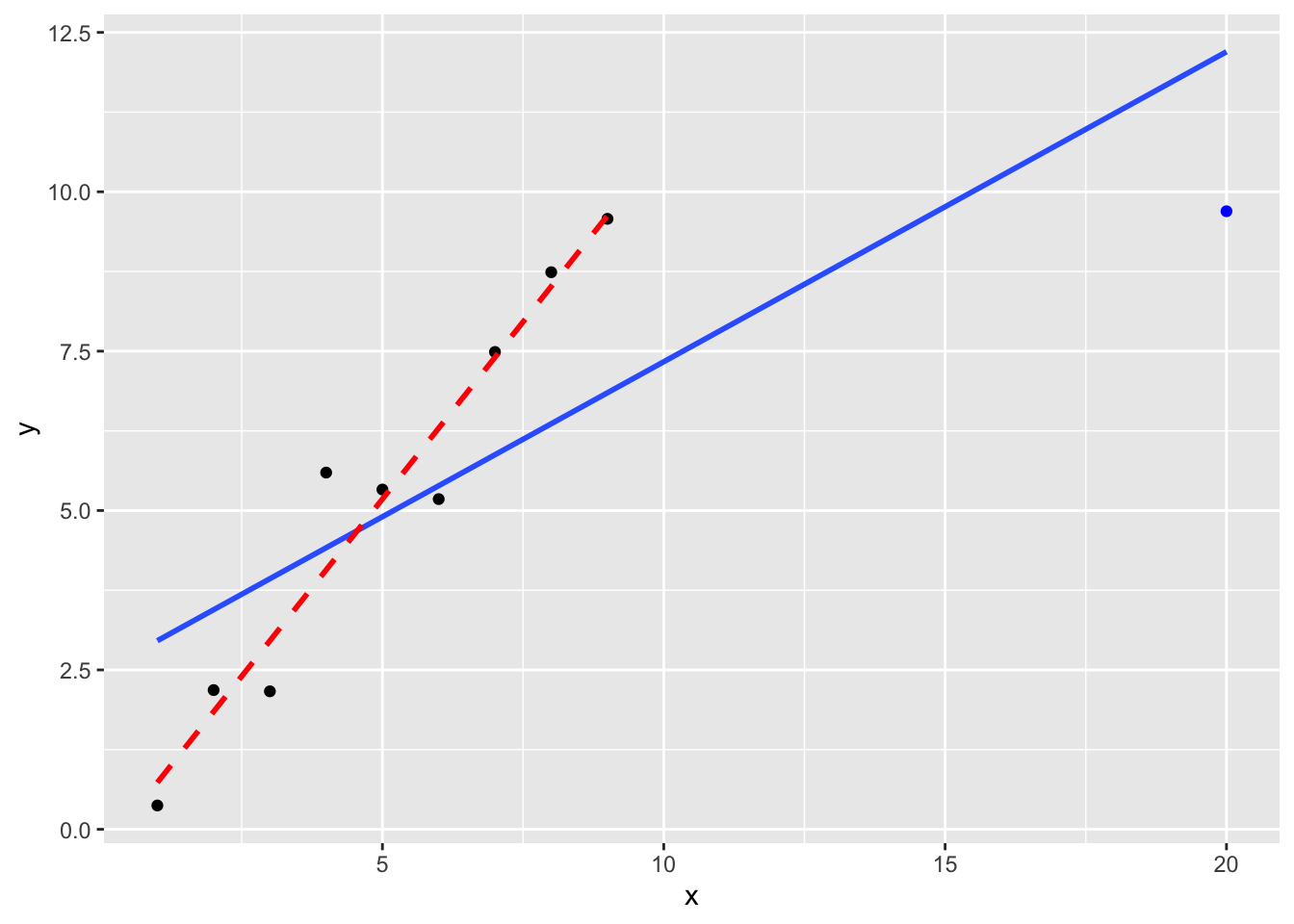
Figure 7.4: The blue line is the least squares fit using all ten observations. The red dashed line is the least squares fit, omitting the ‘high leverage’ point at \(x=20\); the least squares fit will be particularly sensitive to this one observation.
7.3 Relationship with maximum likelihood estimation
Exercise. (This is a good opportunity to test your understanding of likelihood!) Suppose, in the simple linear regression model, \(\beta_0\) and \(\beta_1\) are to be estimated by maximum likelihood. Show that the maximum likelihood estimates are also the least squares estimates. (You will not need to actually obtain the maximum likelihood estimates to prove this: you just need to show that maximum likelihood must result in the same solution.)
Solution
The likelihood function is given by
\[ L(\beta_0, \beta_1, \sigma^2; \mathbf{y}) = \prod_{i=1}^nf_Y(y_i; \beta_0, \beta_1,\sigma^2) \] We have \(Y_i \sim N(\beta_0 + \beta_1x_i, \sigma^2)\), so \[ f_Y(y_i; \beta_0, \beta_1,\sigma^2) = \frac{1}{\sqrt{2\pi\sigma^2}}\exp\left(-\frac{1}{2\sigma^2}(y_i - \beta_0-\beta_1x_i)^2\right) \] and so the log-likelihood is \[ \ell(\beta_0, \beta_1, \sigma^2; \mathbf{y}) = -\frac{n}{2}\log\sigma^2 - \frac{1}{2\sigma^2}\sum_{i=1}^n(y_i - \beta_0-\beta_1x_i)^2. \] The maximum likelihood estimators of \(\beta_0\) and \(\beta_1\) are the solutions of \[\begin{align*} \frac{\partial \ell}{\partial \beta_0} &= \frac{1}{\sigma^2}\sum_{i=1}^n(y_i - \beta_0-\beta_1x_i) = 0,\\ \frac{\partial \ell}{\partial \beta_1} &= \frac{1}{\sigma^2}\sum_{i=1}^nx_i(y_i - \beta_0-\beta_1x_i) = 0, \end{align*}\] but these are the same two simultaneous equations we solved to get the least squares estimates of \(\beta_0\) and \(\beta_1\): the least squares estimates are the same as the maximum likelihood estimates.
7.4 Estimating \(\sigma^2\)
We’ll just state the estimate of \(\sigma^2\), without going too much into the detail. We define \[ \hat{y}_i = \hat{\beta}_0 + \hat{\beta}_1 x_i \] to be the \(i\)-th fitted value, so that \((x_i, \hat{y}_i)\) is a point on the fitted regression line. We define \[ e_i = y_i - \hat{y}_i \] to be the \(i\)-th residual: the difference between the observation \(y_i\) and the corresponding fitted value \(\hat{y}_i\). Informally, we could think of \(e_i = y_i - \hat{\beta}_0 + \hat{\beta}_1 x_i\) as an estimate of the error term \(\varepsilon_i = y_i - \beta_0 + \beta_1 x_i\). We then estimate \(\sigma^2\) using the residual sum of squares \[ \hat{\sigma}^2 = \frac{1}{n-2} \sum_{i=1}^n e_i^2. \] The denominator \(n-2\) is the residual degrees of freedom. Informally, it makes sense that we need at least three observations (for the simple linear regression model) to estimate \(\sigma^2\), because with only two observations, the fitted line would pass through both points; we wouldn’t have any idea how far an observation can be from the regression line.
We can get \(\hat{\sigma}^2\) easily from R, but we will do the calculation manually for now. Repeating the earlier code:
x <- election$machine.diff
y <- election$absentee.diff
beta1Hat <- sum((x - mean(x)) * (y - mean(y)))/
  sum((x - mean(x))^2)
beta0Hat <- mean(y) - beta1Hat * mean(x)
Then
e <- y - beta0Hat - beta1Hat*x
sum(e^2) / (length(e) - 2)
## [1] 105519.8This suggests that most points will be within \(2\sqrt{105519.8}\simeq 650\) of the fitted regression line (on the \(y\)-axis). From looking at panel (b) in Figure 7.2, this seems about right.