In this chapter we will discuss some issues and problems that can arise with hypothesis testing, in particular:
problems with conducting a large number of tests in a single investigation;
correlations between parameter estimators and the consequences for tests;
correlation versus causation.
6.1 Multiplicity
Suppose we have a data set with a large number of independent variables, where the aim is to investigate whether any of them are associated with the dependent variable. For example, in a multiple regression model, \[
Y_i=\beta_0+\beta_1 x_{i1}+\cdots+\beta_rx_{ir}+\varepsilon_i,
\] we might perform \(r\) separate tests of \(H_0:\beta_j=0\) for each of \(j=1,\ldots,r\). The problem here is that the more tests we do, the higher the risk of falsely rejecting a null hypothesis, assuming the number of true nulls increases. We illustrate this with a simulation experiment, in which the true and fitted models are as follows: \[\begin{align}
\mbox{True model: }Y_i &= \beta_0 + \varepsilon_i,\\
\mbox{Fitted model: }Y_i &= \beta_0 + \sum_{j=1}^{100} \beta_j x_{ij}+\varepsilon_i.
\end{align}\]
Given some data, we will test 100 separate hypotheses \(H_0:\beta_j=0\) for each of \(j=1,\ldots,100\). By construction, we will know that \(H_0\) is really true in each case, but for a test of size 0.05, we’d expect to reject the null hypothesis on 5 out of the 100 occasions.
library(tidyverse)# set random seed for reproducibilityset.seed(61004) # Generate and label the data. By construction, all columns are independentdf1 <-data.frame(matrix(rnorm(1000*101), 1000, 101))colnames(df1) <-c("Y", paste0("X", 1:100))# Fit the model will all 100 independent variables# The Y ~ . notation is shorthand for this.lmFull <-lm(Y ~ . , df1)# Extract the p-values of the 100 t-tests, and arrange in ascending ordercm1 <-as_tibble(summary(lmFull)$coefficients)colnames(cm1)[4] <-"pvalue"cm1$variable <-paste0("beta", 0:100)cm1 %>%arrange(pvalue)
In the table above, we’ve arranged the \(p\)-values in ascending order. We can see three \(p\)-values below 0.05 (roughly what we would expect). In particular, the \(p\)-value for the test \[
H_0: \beta_{78}=0
\] is 0.0002 to 4 d.p., which certainly gives the appearance of strong evidence against \(H_0\).
By construction, however, we know there is no relationship between any of the independent variables and the dependent variables. How can we guard against false results such as these? Two strategies are as follows.
6.1.1 Use a single \(F\)-test
We need to consider the aim of the investigation. In the example above, we might suppose that the investigator was searching for anything associated with the dependent variable, from a large set of candidate variables. The investigator didn’t single out a particular variable (e.g. the \(x_{78}\) variable) in advance of the experiment as the variable most likely to be associated with the dependent variable.
In this scenario, we might test the single hypothesis that none of the variables are associated with the dependent variable: \[
H_0: \beta_1=\beta_2=\ldots=\beta_{100}=0,
\] which we can test with an \(F\)-test: we compare the full model above with a reduced model \[
Y_i = \beta_0 + \varepsilon_i
\] If we do this in R, we find that there is no evidence against \(H_0\):
We refer to collection of tests (such as testing \(H_0:\beta_i=0\) separately for \(i=1,\ldots,100\)) as a family of tests, and we consider family-wise error rates. The family-wise Type I error rate (FWER) would be the probability of falsely rejecting any null hypothesis within the family, out of all cases in which the null hypothesis is true.
The idea is to specify the FWER (e.g. at 0.05), and then adjust the size of each test within the family to achieve (or bound) the FWER. Two possible adjustments are as follows.
Bonferroni correction. If we perform \(n\) tests, and we desire a family-wise Type I error rate of \(\alpha\), we set the size of each individual test to be \(\alpha/n\).
Šidák correction. If we perform \(n\) tests, and we desire a family-wise Type I error rate of \(\alpha\), we set the size of each individual test to be \(\alpha^*:=1-(1-\alpha)^\frac{1}{n}\).
Suppose the null hypothesis is true for all \(n\) tests. For the Bonferroni correction, we have \[
P(\mbox{reject at least one null}) \le \sum_{i=1}^n P(\mbox{reject null in $i$-th test}) = n\frac{\alpha}{n} = \alpha
\] For the Šidák correction, assuming the test outcomes are independent\[
P(\mbox{reject at least one null}) =1-P(\mbox{do not reject any null}) = 1-(1-\alpha^*)^n = \alpha
\] Hence the Šidák correction gives an exact FWER of \(\alpha\), under an assumption of independent tests. The Bonferroni correction only given an upper bound for the FWER, but does not assume independent tests.
Note
The two corrections give very similar values. If you ever find that your result depends upon which you use, then I’d encourage you to consider the following quote from the mathematician Richard Hamming (which I think is relevant in many situations!)
“Does anyone believe that the difference between the Lebesgue and Riemann integrals can have physical significance, and that whether say, an airplane would or would not fly could depend on this difference? If such were claimed, I should not care to fly in that plane.”
In the example with 100 tests, for a target FWER of 0.05, we’d look for a \(p\)-value smaller than 0.0005, and for a target FWER of 0.01, we’d look for a \(p\)-value smaller than 0.0001. The smallest \(p\)-value we observed was 0.00017, so we’d be more sceptical that we have found a genuine association.
6.2 Small effect sizes: significance versus importance
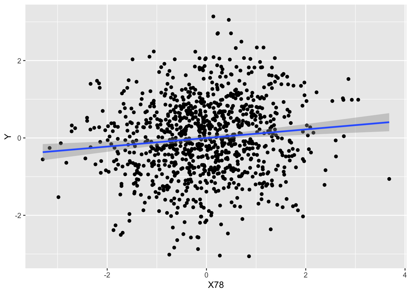
It’s important not to get too carried away with a significant result! The effect size may be too small for the result to have any practical importance. Continuing the example above, \(R^2_{adj}\) is very small, about 2%:
summary(lmFull)$adj.r.squared
[1] 0.02055728
and a scatter plot of the dependent variable against \(x_{78}\) shows mostly random scatter and a relatively shallow gradient in the fitted line
ggplot(df1, aes(x = X78, y = Y)) +geom_point()+geom_smooth(method ="lm")
6.3 Relationships between independent variables
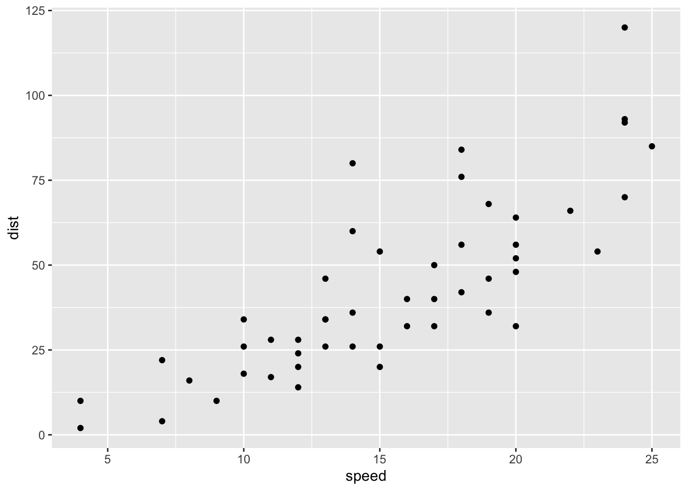
Consider the following example using the cars data. We’d clearly expect there to be a relationship between speed and stopping distance, and it is visible in a scatter plot:
ggplot(cars, aes(x = speed, y = dist)) +geom_point()
Call:
lm(formula = dist ~ speed + I(speed^2), data = cars)

Residuals:
    Min      1Q  Median      3Q     Max
-28.720  -9.184  -3.188   4.628  45.152

Coefficients:
            Estimate Std. Error t value Pr(>|t|)
(Intercept)  2.47014   14.81716   0.167    0.868
speed        0.91329    2.03422   0.449    0.656
I(speed^2)   0.09996    0.06597   1.515    0.136

Residual standard error: 15.18 on 47 degrees of freedom
Multiple R-squared:  0.6673,    Adjusted R-squared:  0.6532
F-statistic: 47.14 on 2 and 47 DF,  p-value: 5.852e-12
The F-statistic shows strong evidence against a null model \(Y_i=\beta_0 + \varepsilon_i\), but in the Coefficients table, neither the coefficients for speed or speed^2 are significant. What is going on here?
Our quadratic regression model is \[
Y_i=\beta_0 + \beta_1x_i + \beta_2x_i^2+ \varepsilon_i.
\]
The issue here is the relationship between \(x_i\) and \(x_i^2\), which is quite close to linear for the given set of \(x_i\) values:
cor(cars$speed, cars$speed^2)
[1] 0.9794765
This means we have two columns in the design matrix \(X\) that are close to being linearly dependent (sometimes referred to as multicollinearity). Intuitively, this suggests that, for the purpose of explaining variation in the dependent variable, we need at most one of \(x_i\) or \(x_i^2\) in our model, but not both: the two variables are, in effect, describing the same thing.
6.3.1 Correlations between estimators
Continuing the example, we have strong correlations between the estimators \(\hat{\beta}_0\), \(\hat{\beta}_1\) and \(\hat{\beta}_2\), and it is helpful to understand what effect this has on model fitting and hypothesis testing.
Recall that \[
Var(\hat{\boldsymbol{\beta}}) = \sigma^2(X^TX)^{-1}
\] We can extract \(X\) from R using the model.matrix() command (and we also use cov2cor() to convert a covariance matrix to a correlation matrix):
The consequence of this is that adding/removing one term (e.g. the term corresponding to \(\beta_1\)) will change the estimated coefficient(s) corresponding to the other term(s).
Tip
Check this for yourself. Investigate what happens to the coefficients as terms are added or removed: try fitting models such as
and comparing the estimated coefficients in each case.
This gives us another way to understand why the individual \(t\)-tests were not significant. For example, if we consider a test of \(\beta_1=0\), we can think of this as a model comparison between \[\begin{align}
\mbox{full model: }Y_i&=\beta_0 + \beta_1x_i + \beta_2x_i^2+ \varepsilon_i,\\
\mbox{reduced model: }Y_i&=\beta_0 + \beta_2x_i^2+ \varepsilon_i.
\end{align}\]
Note
The fitted full model coefficients are obtained as follows:
In comparing the full and reduced model, we are not comparing \[\begin{align}
\mbox{full model: }Y_i&=2.47 + 0.91x_i + 0.10x_i^2+ \varepsilon_i,\\
\mbox{reduced model: }Y_i&=2.47 + 0.10x_i^2+ \varepsilon_i.
\end{align}\] When we fit the reduced model to the data, the estimates of \(\beta_0\) and \(\beta_2\) will change, because of the correlation between the least squares estimators. In this case, the fact that the estimate change result in the reduced model fitting nearly as well as the full model. We can see this by noting the residual sum of squares for each model in the following:
Analysis of Variance Table

Model 1: dist ~ I(speed^2)
Model 2: dist ~ speed + I(speed^2)
  Res.Df   RSS Df Sum of Sq      F Pr(>F)
1     48 10871
2     47 10825  1    46.423 0.2016 0.6555
Exercise
Exercise 6.1 In the example above, suppose the reduced model was fitted simply by setting \(\hat{\beta}_1=0\) in the full model; the other parameter estimates don’t change. In R, lmQuad$fitted.values will extract the fitted values for the full model. Compare the residual sum of squares for the two models, if the reduced model was fitted in this way.
Solution
In this case, we subtract \(\hat{\beta}_1x_i\) from the \(i\)-th fitted value in the full model
Using these ‘wrong’ fitted values, the residual sum of squares would be
sum((yhatWrong - cars$dist)^2)
[1] 21858.17
which is about double the residual sum of squares for the full model.
For designed experiments (where we can choose the dependent variable values), it can be desirable to aim for orthogonal columns in the design matrix, such that parameter estimators are independent, making it easier to isolate the effect of individual variables. (much more on this in the Sampling and Design module). In this particular example, we could make use of orthogonal polynomials. This is outside the scope of this model, but there is brief discussion in the Chapter appendix for anyone interested.
6.4 Correlation and causality
You have probably heard the phase “correlation is not the same as causation”. The classic example of this is the scenario of increasing temperatures causing both an increase in ice-cream sales, and an increase in violent crime (through increased alcohol consumption). If we examine ice-cream sales and violent crime together, we might observe correlation between them, but we wouldn’t believe this to be a causal relationship.
Causal inference is an interesting and active research topic, and connects in an intuitive way with linear modelling. A good introduction is given in
We will give a very short discussion here, in the context of hypothesis tests (and parameter estimation) for linear models.
6.4.1 Graphical models
It can be helpful to represent relationships between variables using graphs, with nodes representing variables and directed edges between nodes representing causal relationships.
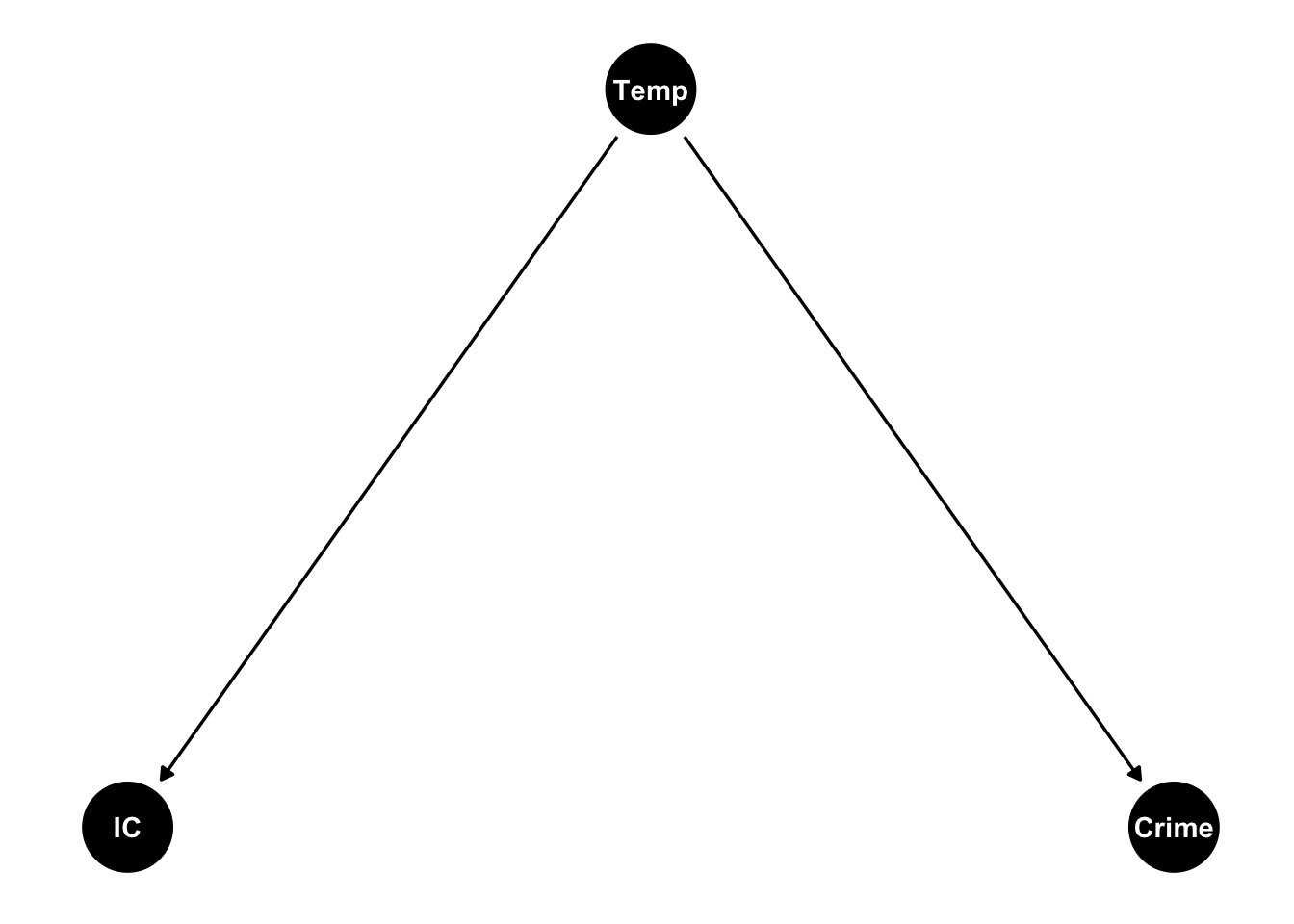
library(dagitty)library(ggdag)dag <-dagitty("dag{ IC <- Temp -> Crime}")coordinates( dag ) <-list( x=c(Temp =1, IC =0, Crime =2),y=c(Temp =1, IC =0, Crime =0) )ggdag(dag) +theme_dag_blank()
In this plot the arrow going from Temp (temperature) to IC (ice cream sales) represents a causal relationship: the volume of ice cream sales is ‘caused’ by the value of the temperature, and potentially other unmeasured variables represented by an error term, e.g. \[
IC_i = \beta_0 + \beta_1Temp_i + \varepsilon_i.
\] The diagram represents a similar causal relationship between temperature and crime, but no causal relationship between ice creams sales and crime. Ice creams sales and crime are correlated, however, due to their common dependence on temperature.
We’ll now consider a few examples of causal relationships versus correlations, and how they might be explored through hypothesis tests.
6.4.2 Conditional independence
In the ice cream example, we might expect ice cream sales and crime to be independent conditional on temperature (the idea of conditional independence is developed more formally in the Bayesian statistics module).
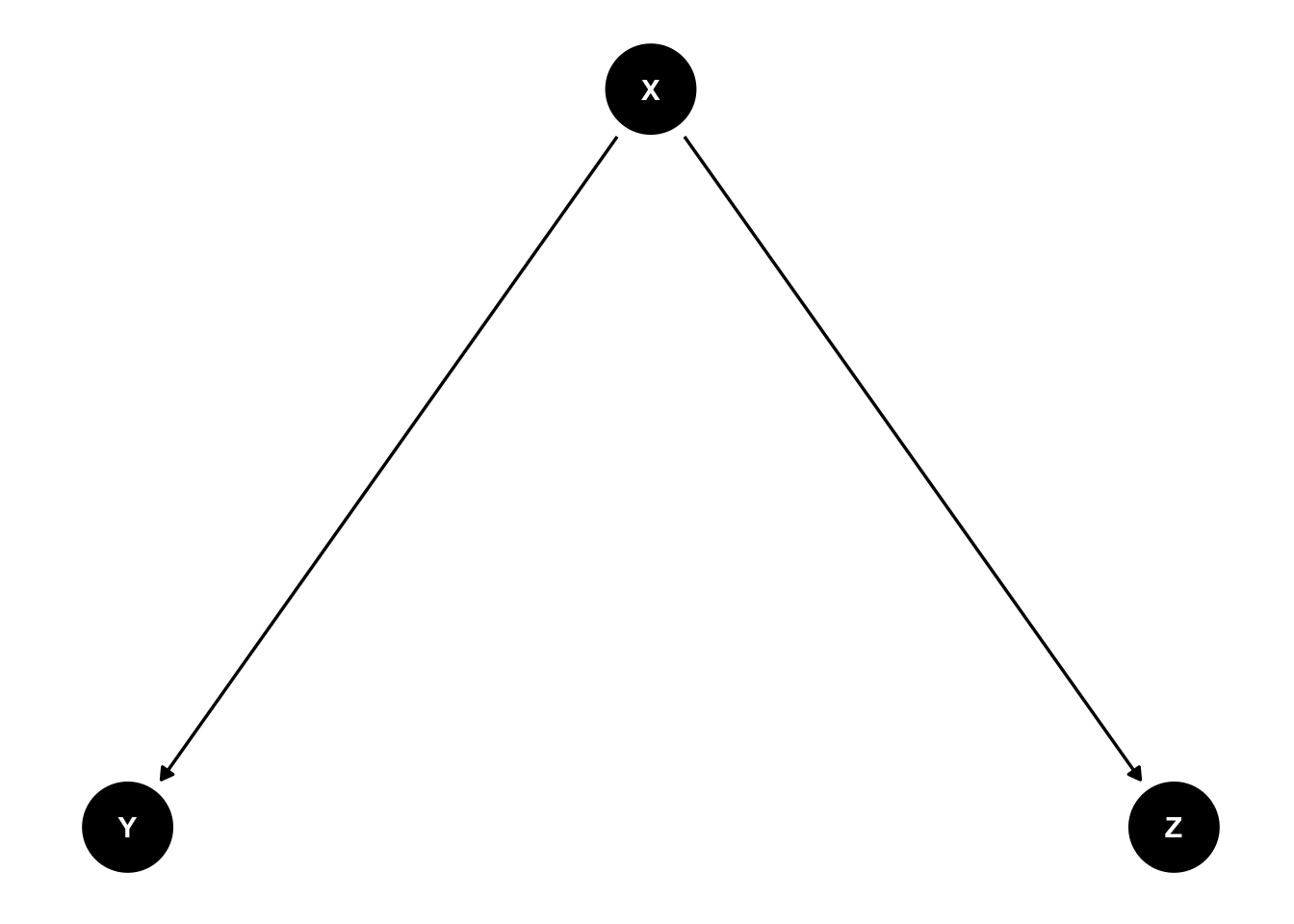
In general, suppose we have three random variables: \(X, Y\) and \(Z\), where both \(Y\) and \(Z\) are dependent on \(X\), but conditionally independent given the value of \(X\). We visualise this as follows:
As an example, suppose that the true ‘causal’ relationships between the variables are given by \[\begin{align}
Y_i &= \beta_0 + \beta_1 X_i + \varepsilon_i,\\
Z_i &= \alpha_0 + \alpha_1 X_i + \delta_i,\\
\end{align}\] where \(\varepsilon_i\) and \(\delta_i\) are random error terms. We’ll first generate some random data in R:
set.seed(61004)x <-1:100y <- x +rnorm(100)z <- x +rnorm(100)
If we try a simple linear regression model of \(Y\) on \(Z\), we would detect a relationship between \(Y\) and \(Z\):
lmYonZ <-lm(y ~ z)summary(lmYonZ)
Call:
lm(formula = y ~ z)

Residuals:
    Min      1Q  Median      3Q     Max
-3.3232 -0.8955 -0.1176  0.8613  3.2355

Coefficients:
            Estimate Std. Error t value Pr(>|t|)
(Intercept) 0.010668   0.291562   0.037    0.971
z           0.999672   0.005003 199.811   <2e-16 ***
---
Signif. codes:  0 '***' 0.001 '**' 0.01 '*' 0.05 '.' 0.1 ' ' 1

Residual standard error: 1.449 on 98 degrees of freedom
Multiple R-squared:  0.9976,    Adjusted R-squared:  0.9975
F-statistic: 3.992e+04 on 1 and 98 DF,  p-value: < 2.2e-16
However, if we include the variable \(X\) in our model, the evidence for a relationship between \(Y\) and \(Z\) disappears:
lmYonXandZ <-lm(y ~ x + z)summary(lmYonXandZ)
Call:
lm(formula = y ~ x + z)

Residuals:
     Min       1Q   Median       3Q      Max
-2.55853 -0.53880  0.09033  0.58057  2.75507

Coefficients:
            Estimate Std. Error t value Pr(>|t|)
(Intercept) -0.11805    0.19322  -0.611    0.543
x            1.09501    0.09720  11.266   <2e-16 ***
z           -0.09123    0.09689  -0.942    0.349
---
Signif. codes:  0 '***' 0.001 '**' 0.01 '*' 0.05 '.' 0.1 ' ' 1

Residual standard error: 0.9585 on 97 degrees of freedom
Multiple R-squared:  0.9989,    Adjusted R-squared:  0.9989
F-statistic: 4.567e+04 on 2 and 97 DF,  p-value: < 2.2e-16
Note
If we want to investigate the relationship between \(Y\) and \(Z\), and suspect they are both dependent on a third variable \(X\), we should adjust for that variable in our modelling: we include \(X\) as in independent variable in the model, and then see whether including \(Z\) as an additional independent variable improves our ability to predict \(Y\).
6.4.3 Post-treatment variables
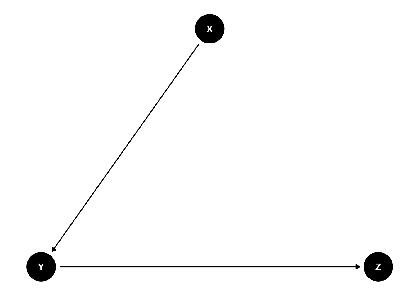
A different scenario is where we a variable \(X\) has a causal effect on our dependent variable \(Y\), and the dependent variable \(Y\) has a causal effect on some other quantity \(Z\). For example, for an individual exercise (\(X\)) might cause weight loss (\(Y\)), which might then result in a cholesterol reduction (\(Z\)). We would refer to cholesterol reduction as a post-treatment variable in that it isn’t determined until after the treatment \(X\) has been applied and the effect on \(Y\) determined. The graphical representation would be as follows:
This has implications for what should be included in a model. We suppose that the true ‘causal’ relationships between the variables are given by \[\begin{align}
Y_i &= \beta_0 + \beta_1 X_i + \varepsilon_i,\\
Z_i &= \alpha_0 + \alpha_1 Y_i + \delta_i,\\
\end{align}\] where \(\varepsilon_i\) and \(\delta_i\) are random error terms. We’ll first generate some random data in R (with \(\beta_0=0\) and \(\beta_1=1\)):
set.seed(61004)x <-seq(from =0, to =10, length =100)y <- x +rnorm(100, 0, 1)z <- y +rnorm(100, 0, 1)
A simple linear regression of \(Y\) on \(X\) will give estimates of \(\beta_0\) and \(\beta_1\) close to their true values:
lmYonX <-lm(y ~ x)summary(lmYonX)
Call:
lm(formula = y ~ x)

Residuals:
    Min      1Q  Median      3Q     Max
-2.5438 -0.5781  0.0856  0.6364  2.6931

Coefficients:
            Estimate Std. Error t value Pr(>|t|)
(Intercept) -0.10914    0.19015  -0.574    0.567
x            1.03513    0.03285  31.508   <2e-16 ***
---
Signif. codes:  0 '***' 0.001 '**' 0.01 '*' 0.05 '.' 0.1 ' ' 1

Residual standard error: 0.9579 on 98 degrees of freedom
Multiple R-squared:  0.9102,    Adjusted R-squared:  0.9092
F-statistic: 992.7 on 1 and 98 DF,  p-value: < 2.2e-16
Now observe how including the post-treatment variable \(Z\) in the model changes the estimated effect of the treatment \(X\):
lmYonXandZ <-lm(y ~ x + z)summary(lmYonXandZ)
Call:
lm(formula = y ~ x + z)

Residuals:
     Min       1Q   Median       3Q      Max
-1.64776 -0.47647 -0.03676  0.38458  1.62566

Coefficients:
            Estimate Std. Error t value Pr(>|t|)
(Intercept) -0.03031    0.14468  -0.209    0.835
x            0.52946    0.06423   8.243 8.17e-13 ***
z            0.47666    0.05580   8.543 1.86e-13 ***
---
Signif. codes:  0 '***' 0.001 '**' 0.01 '*' 0.05 '.' 0.1 ' ' 1

Residual standard error: 0.7273 on 97 degrees of freedom
Multiple R-squared:  0.9487,    Adjusted R-squared:  0.9477
F-statistic: 897.4 on 2 and 97 DF,  p-value: < 2.2e-16
Note
Including the post-treatment variable in the regression model changes the objective of the regression model: the implied objective is to find the best prediction of \(Y\) given both \(X\) and \(Z\), not to reveal the causal relationship between \(Y\) and \((X,Z)\). If the real purpose is to predict \(Y\) given \(X\) only, we should not include \(Z\) in the model.
6.5 Replication
Although outside the scope of what we can do in this module, it is important to consider replicating any study to see if the same result is obtained. The replicability of scientific findings is itself now an active area of research. See for example
Camerer, C.F., Dreber, A., Holzmeister, F. et al. (2018) Evaluating the replicability of social science experiments in Nature and Science between 2010 and 2015. Nat Hum Behav 2, 637–644 . https://doi.org/10.1038/s41562-018-0399-z
Ioannidis J.P.A. (2005) Why Most Published Research Findings Are False. PLoS Med 2(8): e124. https://doi.org/10.1371/journal.pmed.0020124 pmid:16060722]
In clinical trials for new medicines, regulators such as the US Food and Drug Administration and the European Medicines Agency may require two (Phase III) studies demonstrating the effectiveness of a drug.
6.6 Chapter appendix
The following topic is outside the scope of this module, but is included for interest.
6.6.1 Orthogonal polynomials
In the example in Section 6.3, we can use orthogonal polynomials. The idea is to use Gram-Schmidt orthogonalisation to transform the columns of the design matrix \(X\) to set of linearly independent (orthogonal) columns. This makes the coefficients harder to interpret, but it is then possible to isolate a quadratic effect, if we were interested in testing for it. (It can also improve numerical stability of the results.)
We use the poly() command to set up orthogonal polynomials. We’ll compare quadratic regression models using both raw and orthogonal polynomials
# Using raw polynomialslmRaw <-lm(dist ~ speed +I(speed^2), cars)# Using orthogonal polynomialslmOrthogonal <-lm(dist ~poly(speed, degree =2), cars)
summary(lmRaw)
Call:
lm(formula = dist ~ speed + I(speed^2), data = cars)

Residuals:
    Min      1Q  Median      3Q     Max
-28.720  -9.184  -3.188   4.628  45.152

Coefficients:
            Estimate Std. Error t value Pr(>|t|)
(Intercept)  2.47014   14.81716   0.167    0.868
speed        0.91329    2.03422   0.449    0.656
I(speed^2)   0.09996    0.06597   1.515    0.136

Residual standard error: 15.18 on 47 degrees of freedom
Multiple R-squared:  0.6673,    Adjusted R-squared:  0.6532
F-statistic: 47.14 on 2 and 47 DF,  p-value: 5.852e-12
summary(lmOrthogonal)
Call:
lm(formula = dist ~ poly(speed, degree = 2), data = cars)

Residuals:
    Min      1Q  Median      3Q     Max
-28.720  -9.184  -3.188   4.628  45.152

Coefficients:
                         Estimate Std. Error t value Pr(>|t|)
(Intercept)                42.980      2.146  20.026  < 2e-16 ***
poly(speed, degree = 2)1  145.552     15.176   9.591 1.21e-12 ***
poly(speed, degree = 2)2   22.996     15.176   1.515    0.136
---
Signif. codes:  0 '***' 0.001 '**' 0.01 '*' 0.05 '.' 0.1 ' ' 1

Residual standard error: 15.18 on 47 degrees of freedom
Multiple R-squared:  0.6673,    Adjusted R-squared:  0.6532
F-statistic: 47.14 on 2 and 47 DF,  p-value: 5.852e-12
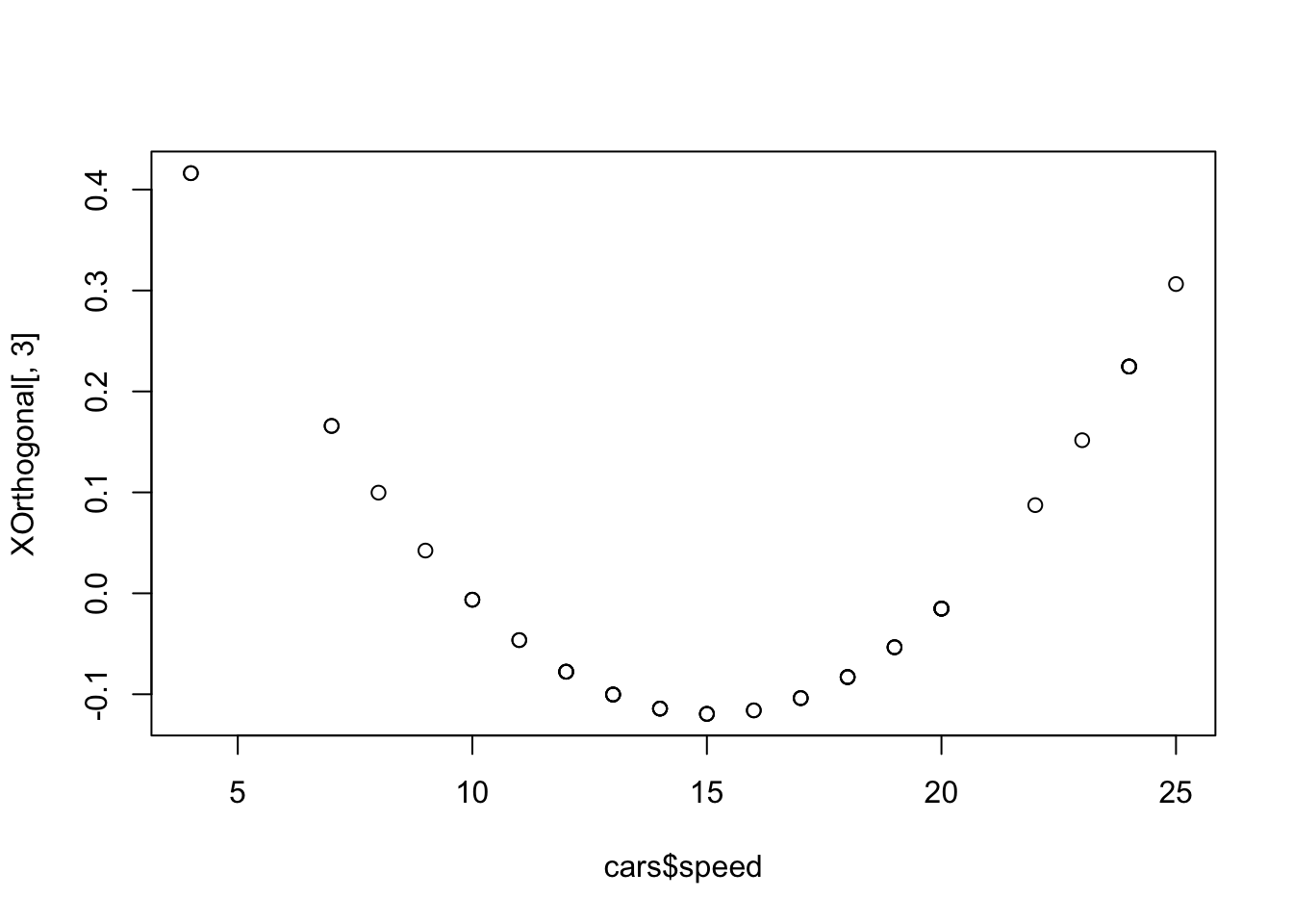
Note that the residual standard error and \(R^2\) statistics are the same for both versions: switching to orthogonal polynomials doesn’t improve the model fit. But in the orthogonal case, we see that the linear term is significant; the quadratic term is not.
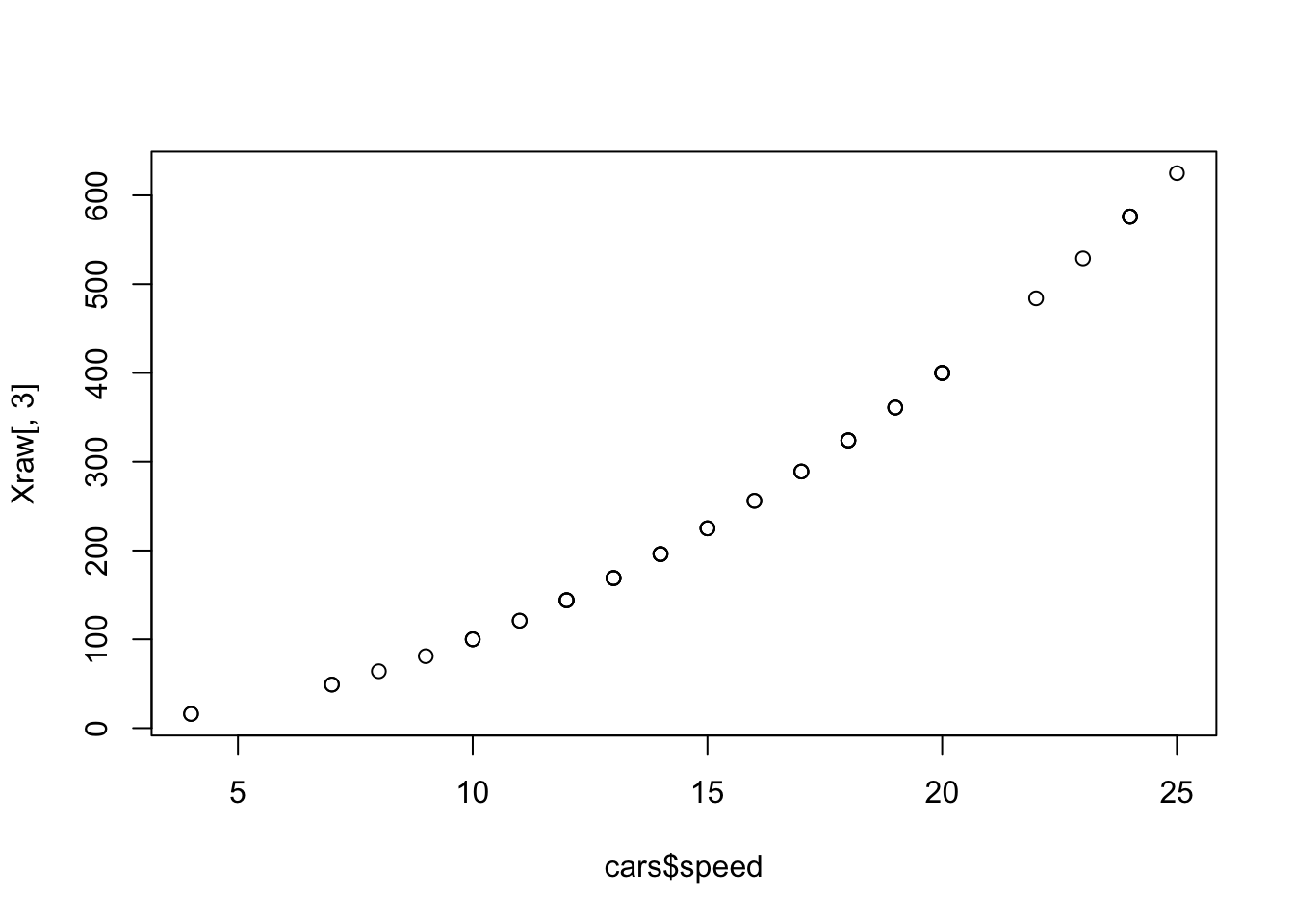
Note that the off-diagonal elements in the orthogonal polynomial model are all very close to 0 (rounding errors): the parameter estimators are all independent. Finally, to help visualise the quadratic term using orthogonal polynomials, we’ll plot the third column of the design matrix \(X\) each model against speed