8  Transformations

In the previous chapter we looked at checking model assumptions. In this chapter we consider what to do if the model assumptions do not hold, specifically the assumption that the error variance is constant.

8.1 Transforming to restore homoscedasticity

8.1.1 Theory

We usually transform the dependent variable when we suspect, either by doing diagnostic checks on residuals or for some other reason, that the model assumption of homoscedasticity does not hold. An alternative approach could be to try a Generalised Linear Model, which is often particularly suitable if there are reasons to suggest a distribution other than the Normal would be a better model; this will be covered in a later component of this module.

Suppose that \(Y\) is a random variable whose variance depends on its mean, so that if \(E(Y)=\mu\) then \(Var(Y)=g(\mu)\), and the function \(g\) is known. (For example, a Poisson random variable has variance equal to its mean.) We seek a transformation from \(Y\) to \(Z=f(Y)\) such that the variance of \(Z\) is (approximately) constant. This is known as a variance-stabilizing transformation.

Consider expanding \(f\) in a Taylor series about its mean. Keeping only the first order term, we have \[ z=f(y)\approx f(\mu)+(y-\mu)f'(\mu). \] Now taking expectations of \(Z=f(Y)\), \[\begin{align} E(Z)&\approx E(f(\mu)+(Y-\mu)f'(\mu))\\ &=f(\mu)+(E(Y)-\mu)f'(\mu)\\ &=f(\mu) \end{align}\] and since \(f'(\mu)\) is a scalar \[\begin{align} Var(Z)&\approx Var(Yf'(\mu))\\ &=Var(Y)(f'(\mu))^2\\ &=g(\mu)(f'(\mu))^2. \end{align}\] We want this to be a constant, \(k^2\) say, so that \(k^2=g(\mu)f'(\mu)^2\). Therefore we seek a function \(f\) such that \[ f'(\mu)=\frac{k}{\sqrt{g(\mu)}}. \] Therefore the solution is \[ f(\mu)=k\int (g(\mu))^{-1/2}\,d\mu. \]

Example 8.1 Variance proportional to mean

Suppose that the variance is proportional to the mean, so that \(g(\mu)=a\mu\). Then \[ f(\mu)=ka^{-1/2}\int \mu^{-1/2}\,d\mu=2ka^{-1/2}\sqrt{\mu}+C. \]

Since \(C\), \(k\) and \(a\) are arbitrary constants, a variable of the form \(Z=A\sqrt{Y}+C\) should have approximately constant variance, with the most obvious choice perhaps being \(Z=\sqrt{Y}\). Whether it does depends on how accurate our estimation of the function \(g\) is (i.e. our assessment of how the variance of the response depends on the mean). If we are assessing this relationship by eye it may not be very accurate.

Example 8.2 Standard deviation proportional to mean

Suppose the standard deviation of \(Y\) is proportional to \(\mu\), so that \(g(\mu)=a\mu^2\), then \[ f(\mu)=ka^{-1/2}\int \mu^{-1}\,d\mu=ka^{-1/2} \log \mu+C. \] The transformed variable \(Z=\log Y\) should have approximately constant variance.

8.1.2 Determining how the variance depends on the mean

Inspecting a plot of \(e_i\) against \(\hat{y}_i\) is a common way to check for non-homoscedasticity. If we see a funnel shape with the spread of the residuals seeming to increase linearly with \(\hat{y}_i\), then this suggests that the standard deviation of \(y_i\) is proportional to its mean. Then, Example 8.2 above suggests that we should use a log transformation.

If we see signs of increasing standard deviation, but the growth flattens out as \(y_i\) increases, this suggests something more like the variance being proportional to the mean. Then Example 8.1 above suggests using a square root transformation of the dependent variable.

Other patterns might suggest other kinds of \(g(\mu)\), although in practice it is hard to distinguish anything more subtle unless we have a large data set.

Remember that in terms of the transformed variable, what may have been a linear relationship between \(y\) and the regressor variables becomes a nonlinear relationship between the new \(z\) and the same regressor variables. This can mean that although a linear model for \(z\) better satisfies the assumption of homoscedasticity we cannot represent \(z\) so well through linear combinations of regressor variables. So removing a problem of heteroscedasticity can introduce other problems.

Fortunately, in practice the reverse is often true. We frequently find that after a suitable variance-stabilizing transformation the relationship between the dependent variable and regressor variables actually simplifies. Indeed, the transformation often also improves normality.

8.2 Estimating a transformation

8.2.1 Families of transformations

In a situation where we cannot easily determine how the variance of the response depends on the mean by eye, a formal statistical approach to transformations is to try to estimate what transformation to use.

Suppose that we have a family of transformations \(f_\lambda\) indexed by a parameter \(\lambda\). So for any given \(\lambda\) we could define the new dependent variable \(z_\lambda=f_\lambda(y)\). Suppose that we believe that there is some value of \(\lambda\) for which \(z_\lambda\) follows a linear model in which all the assumptions are true. Then we have a model \[ f_\lambda(y_i)=\boldsymbol{x}_i^T\boldsymbol{\beta}+\varepsilon_i \] where the \(\varepsilon_i\)’s are independent \(N(0,\sigma^2)\). This is a model with parameters \(\boldsymbol{\beta}\), \(\sigma^2\) and \(\lambda\).

8.2.2 Maximum likelihood

We can estimate \(\lambda\) by maximum likelihood. To calculate the likelihood we have to remember that we do not observe \(f_\lambda(y_i)\), which depends on the unknown parameter \(\lambda\). We observe the \(y_i\), and the likelihood should be the joint probability density function of the \(y_i\) given the parameters, and this entails bringing in the derivative of the transformation. The likelihood is \[ L(\boldsymbol{\beta},\sigma^2,\lambda;\boldsymbol{y}) \propto \sigma^{-n} \exp\left\{ -\frac{1}{2\sigma^2}\sum_{i=1}^n \left(f_\lambda(y_i)-\boldsymbol{x}_i^T\boldsymbol{\beta}\right)^2\right\} \prod_{i=1}^n f_\lambda'(y_i). \]

We already know how to maximize the likelihood with respect to and \(\boldsymbol{\beta}\) and \(\sigma^2\), for fixed \(\lambda\). We first choose \(\boldsymbol{\hat{\beta}}\) to minimize the sum of squares in the exponent. The minimal value is the residual sum of squares, which we now denote by \[ S_\lambda:=\sum_{i=1}^n \left(f_\lambda(y_i)-\boldsymbol{x}_i^T\hat{\boldsymbol{\beta}}\right)^2 \] to show that it depends on \(\lambda\). Then the maximization with respect to \(\sigma^2\) yields \(\hat{\sigma}_\lambda^2=S_\lambda/n\). Hence the exponent term in the likelihood, once maximised with respect to \(\boldsymbol{\beta}\) and \(\sigma^2\) is

\[ \exp\left\{ -\frac{1}{2\hat{\sigma}^2}\sum_{i=1}^n \left(f_\lambda(y_i)-\boldsymbol{x}_i^T\hat{\boldsymbol{\beta}}\right)^2\right\} = \exp\left\{-\frac{n}{2S_{\lambda}} S_{\lambda}\right\}, \] which is constant for all \(\lambda\).

We now have \[ L(\boldsymbol{\hat{\beta}}_\lambda,\hat{\sigma}_\lambda^2,\lambda;\boldsymbol{y}) \propto S_\lambda^{-n/2} \prod_{i=1}^n f_\lambda'(y_i). \] The MLE of \(\lambda\) is now obtained by maximising \(L(\boldsymbol{\hat{\beta}}_\lambda,\hat{\sigma}_\lambda^2,\lambda;\boldsymbol{y})\). In practice it is usually easier to maximise its logarithm \[ \ell(\boldsymbol{\hat{\beta}}_\lambda,\hat{\sigma}_\lambda^2,\lambda;\boldsymbol{y}) = c-\frac{n}{2}\log S_\lambda +\sum_{i=1}^n \log f_\lambda'(y_i), \] where \(c\) is a constant (not depending on \(\lambda\)) and can be ignored when maximizing.

8.2.3 The Box-Cox family

Whilst the above theory works for any family of transformations, by far the most popular family is the family of power transformations, also known as the Box-Cox family. Box and Cox (1964) proposed a family of transformations on the response variable to correct non-normality and/or non-constant variance. If the response is positive, the transformation is given by \[ f_\lambda(y)=\left\{\begin{array}{ll}(y^\lambda-1)/\lambda, & \lambda\neq 0 \\ \log y, & \lambda=0\end{array}\right. \] It can be shown that \(f_\lambda(y)\) is a continuous function of \(\lambda\). We assume that the transformed values of \(Y\) are normally distributed about a linear combination of the covariates with constant variance, that is \(f_\lambda(Y_i)\sim N(\boldsymbol{x}_i^T\boldsymbol{\beta},\sigma^2)\) for some unknown value of \(\lambda\). Hence, the problem is to estimate \(\lambda\) as well as the parameter vector \(\boldsymbol{\beta}\).

8.2.4 Obtaining a Box-Cox transformation

We now consider using maximum likelihood methods to investigate the most appropriate Box-Cox transformation to use for the simulated data set.

We have \(f_\lambda(y)=(y^\lambda-1)/\lambda\) so that \(f_\lambda '(y)=y^{\lambda-1}\) and the log likelihood takes the form \[ \ell(\boldsymbol{\hat{\beta}}_\lambda,\hat{\sigma}_\lambda^2,\lambda;\boldsymbol{y}) =c-\frac{n}{2}\log S_\lambda +\sum_{i=1}^n \log f_\lambda'(y_i)= c-\frac{n}{2}\log S_\lambda+(\lambda-1)ny_L, \] where \(ny_L\) is the sum of the logarithms of the observations, \(ny_L=\sum_{i=1}^n \log y_i\) and depends only on the values of the response.

Exercise

Exercise 8.1 The residual sum of squares of a fitted model can be obtained using the anova command, e.g

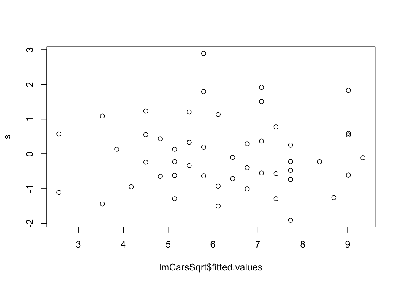
lmCars <- lm(dist ~ speed, cars)
anova(lmCars)
Analysis of Variance Table

Response: dist
          Df Sum Sq Mean Sq F value   Pr(>F)    
speed      1  21186 21185.5  89.567 1.49e-12 ***
Residuals 48  11354   236.5                     
---
Signif. codes:  0 '***' 0.001 '**' 0.01 '*' 0.05 '.' 0.1 ' ' 1

so the residual sum of squares is 11354.

By fitting the models

lm(log(dist) ~ speed, cars)
lm(sqrt(dist) ~ speed, cars)

and using the anova() command to find the residual sum of squares, compare the likelihood values for \(\lambda = 0, 0.5\) and 1, corresponding to a log transformation, a square-root transformation, and no transformation of the dependent variable.

We are given \(S_1=11354\) (the residual sum of squares for no transformation). In R, we do

lmCarsLog <- lm(log(dist) ~ speed, cars)
lmCarsSqrt <- lm(sqrt(dist) ~ speed, cars)
anova(lmCarsLog)
Analysis of Variance Table

Response: log(dist)
          Df  Sum Sq Mean Sq F value    Pr(>F)    
speed      1 19.9804 19.9804   100.3 2.413e-13 ***
Residuals 48  9.5621  0.1992                      
---
Signif. codes:  0 '***' 0.001 '**' 0.01 '*' 0.05 '.' 0.1 ' ' 1
anova(lmCarsSqrt)
Analysis of Variance Table

Response: sqrt(dist)
          Df  Sum Sq Mean Sq F value    Pr(>F)    
speed      1 142.411 142.411  117.18 1.773e-14 ***
Residuals 48  58.334   1.215                      
---
Signif. codes:  0 '***' 0.001 '**' 0.01 '*' 0.05 '.' 0.1 ' ' 1

giving \(S_0 = 9.5621\) and \(S_{0.5} = 58.334\). Computing the three log-likelihood values (ignoring constants), we find

-50/2*log(11354)
[1] -233.4331
-50/2*log(9.5621) - sum(log(cars$dist))
[1] -233.2406
-50/2*log(58.334) - 0.5 * sum(log(cars$dist))
[1] -190.0523

so we have \[\begin{align} \ell(\boldsymbol{\hat{\beta}}_\lambda,\hat{\sigma}_\lambda^2,\lambda = 1;\boldsymbol{y}) &= -233.4,\\ \ell(\boldsymbol{\hat{\beta}}_\lambda,\hat{\sigma}_\lambda^2,\lambda = 0;\boldsymbol{y}) &= -233.2,\\ \ell(\boldsymbol{\hat{\beta}}_\lambda,\hat{\sigma}_\lambda^2,\lambda = 1;\boldsymbol{y}) &= -190.1. \end{align}\]

This suggests that the square root transformation is the best out of the three, and the residual plot does look a little better in this case:

s <- MASS::stdres(lmCarsSqrt)
plot(lmCarsSqrt$fitted.values, s )

In R, we can use the MASS::boxcox() function to plot the profile-likelihood for \(\lambda\):

MASS::boxcox(lm(dist ~ speed, cars),
       lambda=seq(0,1,1/20),
       plotit=TRUE,
       xlab=expression(lambda),
       ylab="Log-likelihood")

If we change the plotit argument to FALSE, we can extract the values in the plot to find the maximum

bc <- MASS::boxcox(lm(dist ~ speed, cars),
                   lambda = seq(0,1,1/20),
                   plotit = FALSE)
bc
$x
 [1] 0.00 0.05 0.10 0.15 0.20 0.25 0.30 0.35 0.40 0.45 0.50 0.55 0.60 0.65 0.70
[16] 0.75 0.80 0.85 0.90 0.95 1.00

$y
 [1] -56.44525 -54.44791 -52.71917 -51.25976 -50.06651 -49.13255 -48.44768
 [8] -47.99897 -47.77145 -47.74884 -47.91427 -48.25086 -48.74223 -49.37287
[15] -50.12839 -50.99563 -51.96275 -53.01918 -54.15560 -55.36382 -56.63671
bc$x[which.max(bc$y)]
[1] 0.45

suggesting an optimal \(\lambda\) around 0.45.

Exercise

Exercise 8.2 Find a suitable Box-Cox transformation for the one-way ANOVA model for the cancer data. Verify that the transformation helps with the model assumptions.

library(tidyverse)
cancer <- read_csv("https://oakleyj.github.io/exampledata/cancer.csv")
lmCancer <- lm(survival ~ organ, cancer)

A bit of trial and error is needed to find an appropriate range of \(\lambda\) values

MASS::boxcox(lmCancer,
             lambda = seq(-0.5, 0.5 ,1/20),
             plotit = TRUE,
             xlab = expression(lambda),
             ylab = "Log-likelihood")

To get the optimal value

bc <- MASS::boxcox(lmCancer,
                   lambda = seq(-0.5, 0.5 ,1/20),
                   plotit = FALSE)
bc
$x
 [1] -0.50 -0.45 -0.40 -0.35 -0.30 -0.25 -0.20 -0.15 -0.10 -0.05  0.00  0.05
[13]  0.10  0.15  0.20  0.25  0.30  0.35  0.40  0.45  0.50

$y
 [1] -161.3377 -158.2974 -155.4732 -152.8754 -150.5141 -148.3997 -146.5426
 [8] -144.9531 -143.6412 -142.6167 -141.8887 -141.4654 -141.3543 -141.5614
[15] -142.0913 -142.9471 -144.1297 -145.6383 -147.4701 -149.6200 -152.0811
bc$x[which.max(bc$y)]
[1] 0.1

We could use the optimal value, though it’s quite close to 0 (a log transformation), so we’ll just try that:

lmCancerLog <- lm(log(survival) ~ organ, cancer)
s <- MASS::stdres(lmCancerLog)
plot(lmCancerLog$fitted.values, s)

We no longer have the funnel shape in the plot, as we would hope.