4  Fitting a linear model and making predictions in R

In this chapter we will

1. fit a simple linear regression model in R;
2. fit models with qualitative independent variables in R (ANOVA and ANCOVA);
3. plot fitted models in R;
4. use the summary() command to extract detailed information about the model fit;
5. derive confidence intervals for mean responses and prediction intervals for individual observations, and see how to calculate these with R

4.1 Fitting a simple linear regression model

To illustrate fitting a linear model in R, for convenience we’ll use one of R’s built in data sets: cars

head(cars)

  speed dist
1     4    2
2     4   10
3     7    4
4     7   22
5     8   16
6     9   10

Our dependent variable (dist) is the stopping distance in feet, and the independent variable is (speed) is the speed in miles per hour. The cars are very old (1920s!), but it’s a convenient data set for illustrating the linear modelling syntax.

The basic syntax is

lm(formula, data )

where the formula argument corresponds to the equation for \(E(Y_i)\) and uses column names from the data frame specified by the data argument. Some formula examples are as follows.

Model	formula
\(Y_i = \beta_0 + \varepsilon_i\)	dist ~ 1
\(Y_i = \beta_0 + \beta_1 x_i+ \varepsilon_i\)	dist ~ speed
\(Y_i = \beta_0 + \beta_1 x_i+ \beta_2 x_i^2+\varepsilon_i\)	dist ~ speed + I(speed^2)
\(Y_i = \beta_0 + \beta_1 \log x_i+\varepsilon_i\)	dist ~ log(speed)

For example, to fit the simple linear regression model we do

lm(dist ~ speed, cars)

Call:
lm(formula = dist ~ speed, data = cars)

Coefficients:
(Intercept)        speed  
    -17.579        3.932  

and from the Coefficients output we read off \(\hat{\beta}_0= -17.579\) and \(\hat{\beta}_1 = 3.932\).

Tip

When studying a topic such as this and trying out R functions, sometimes it can help you to understand what is going on if you can obtain the same results for yourself. For example:

# Setup the design matrix X
X <- matrix(c(rep(1, 50), cars$speed),
            nrow = 50,
            ncol = 2)
# Setup the observation vector
y <- matrix(cars$dist,
            nrow = 50,
            ncol = 1)
# Compute the least squares estimates and compare with the Coefficients output above
solve(t(X) %*% X) %*% t(X) %*% y

           [,1]
[1,] -17.579095
[2,]   3.932409

4.2 Viewing a fitted regression model

We can plot the fitted model and the data with the commands

library(tidyverse)
ggplot(cars, aes(x = speed, y = dist))+
  geom_point()+
  geom_smooth(method = "lm", formula = "y ~ x", se = FALSE)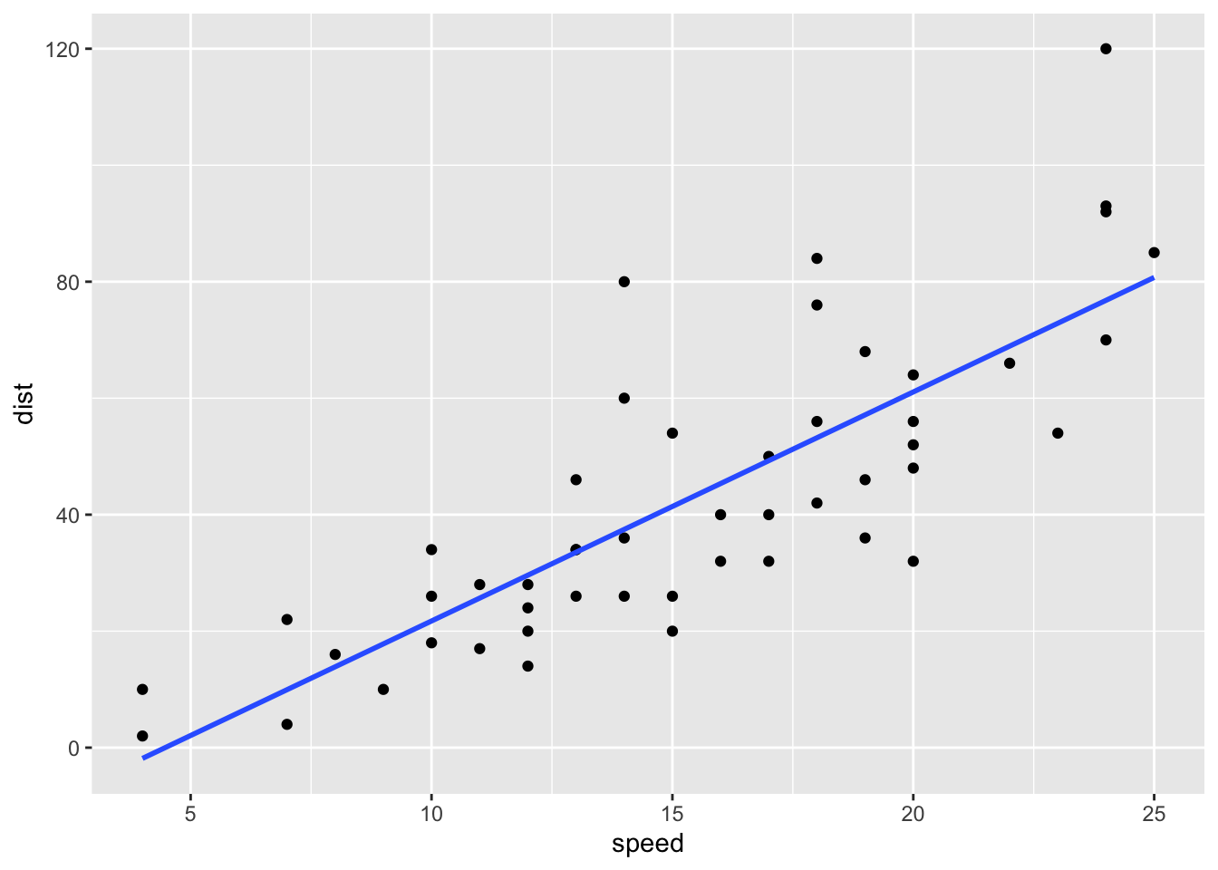

Note that the formula argument corresponds to the fitted model, but with variables x and y rather than speed and dist. We will change the argument se to TRUE when we have learned more about confidence intervals in the next chapter.

4.3 The summary() command

The summary command will give us more information about our model fit, if we first assign the fitted model to a variable.

For example:

lmCars <- lm(dist ~ speed, cars)
summary(lmCars)

Call:
lm(formula = dist ~ speed, data = cars)

Residuals:
    Min      1Q  Median      3Q     Max 
-29.069  -9.525  -2.272   9.215  43.201 

Coefficients:
            Estimate Std. Error t value Pr(>|t|)    
(Intercept) -17.5791     6.7584  -2.601   0.0123 *  
speed         3.9324     0.4155   9.464 1.49e-12 ***
---
Signif. codes:  0 '***' 0.001 '**' 0.01 '*' 0.05 '.' 0.1 ' ' 1

Residual standard error: 15.38 on 48 degrees of freedom
Multiple R-squared:  0.6511,    Adjusted R-squared:  0.6438 
F-statistic: 89.57 on 1 and 48 DF,  p-value: 1.49e-12

We interpret the output as follows.

• Residuals refer to those residuals we defined previously: \(e_i = y_i - \hat{y}_i\).

• The Estimate column gives the least squares estimate.

• The Std. Error column gives the estimated standard error for each least squares estimate.

• The t value and Pr(>|t|) refer to a hypothesis test that the corresponding model parameter is 0. We’ll discuss this in more detail in a later chapter.

• The residual standard error is the estimated value \(\hat{\sigma}\) of \(\sigma\) (standard deviation of the errors, not the variance). Recall that this is computed using the residual sum of squares: \(\hat{\sigma}^2 = \mathbf{e}^T\mathbf{e}/(n-p)\)

• The Multiple R-squared and Adjusted R-squared both report how ‘useful’ the model is for predicting the dependent variable: they report the proportion of the variation in \(y_1,\ldots,y_n\) that can be explained by variation in the dependent variables. The Adjusted R-squared corrects for the number of independent variables in the model.

• The F-statistic and p-value also refer to a hypothesis test which we will discuss later.

Exercise

Exercise 4.1 If you are comfortable with working with matrices and vectors in R, see if you can compute the residual standard error reported in the summary() output above using matrix notation in R.

Solution

# Setup the design matrix X
X <- matrix(c(rep(1, 50), cars$speed),
            nrow = 50,
            ncol = 2)

# Setup the observation vector
y <- matrix(cars$dist,
            nrow = 50,
            ncol = 1)

# Compute the least squares estimates 
betahat <- solve(t(X) %*% X) %*% t(X) %*% y

# Compute the residual vector
e <- y - X %*% betahat

# Residual standard error is (noting n - p = 50 - 2)
sqrt(t(e) %*% e / 48)

         [,1]
[1,] 15.37959

4.4 Models with factor variables

Recall the cancer example from the previous chapter

library(tidyverse)
cancer <- read_csv("https://oakleyj.github.io/exampledata/cancer.csv")
head(cancer)

# A tibble: 6 × 2
  survival organ  
     <dbl> <chr>  
1      124 Stomach
2       42 Stomach
3       25 Stomach
4       45 Stomach
5      412 Stomach
6       51 Stomach

We defined \(Y_{ij}\) as the \(j\)-th observation (survival time) in group \(i\), with group defined by organ (one of stomach, bronchus, colon, ovary or breast)

We fit the model \[ Y_{ij}=\mu_i + \varepsilon_{ij},\] for \(i=1,\ldots,g\), \(j=1,\ldots,n_i\) to the cancer data as follows.

lmCancer <- lm(survival ~ organ - 1, cancer)

(the reason for the - 1 in the formula will become clearer shortly.)

We can now use the summary() command to get the parameter estimates

summary(lmCancer)

Call:
lm(formula = survival ~ organ - 1, data = cancer)

Residuals:
     Min       1Q   Median       3Q      Max 
-1371.91  -241.75  -111.50    87.19  2412.09 

Coefficients:
              Estimate Std. Error t value Pr(>|t|)    
organBreast     1395.9      201.9   6.915 3.77e-09 ***
organBronchus    211.6      162.4   1.303  0.19764    
organColon       457.4      162.4   2.817  0.00659 ** 
organOvary       884.3      273.3   3.235  0.00199 ** 
organStomach     286.0      185.7   1.540  0.12887    
---
Signif. codes:  0 '***' 0.001 '**' 0.01 '*' 0.05 '.' 0.1 ' ' 1

Residual standard error: 669.5 on 59 degrees of freedom
Multiple R-squared:  0.5437,    Adjusted R-squared:  0.505 
F-statistic: 14.06 on 5 and 59 DF,  p-value: 4.766e-09

We have \(\hat{\beta}_1 = 1395.9\), \(\hat{\beta}_2 = 211.6\) and so on.

Warning

Be careful with datasets where a factor/qualitative variable has been recorded numerically! You will need to make sure R understands that the variable is really a factor and not a quantitative variable.

As an example, suppose the cancer data were coded as 1 = Stomach, 2 = Bronchus, 3 = Colon, 4 = Ovary, 5 = Breast. We’ll set up a variable organ2 to represent this:

cancer2 <- cancer %>%
  mutate(organ2 = rep(1:5, times = c(13, 17, 17, 6, 11)))

Now we’ll try

lm(survival ~ organ2, data = cancer2)

Call:
lm(formula = survival ~ organ2, data = cancer2)

Coefficients:
(Intercept)       organ2  
     -240.3        288.9  

What model has been fitted, what does the coefficient organ2 represent here, and why doesn’t it make sense?

We can get R to interpret the organ2 variable correctly, by specifying it as a factor variable:

lm(survival ~ factor(organ2) - 1, data = cancer2)

Call:
lm(formula = survival ~ factor(organ2) - 1, data = cancer2)

Coefficients:
factor(organ2)1  factor(organ2)2  factor(organ2)3  factor(organ2)4  
          286.0            211.6            457.4            884.3  
factor(organ2)5  
         1395.9  

4.4.1 An alternative parameterisation

Recall the alternative parametrisation: \[ Y_{i,j}=\mu + \tau_i + \varepsilon_{i,j}, \] for \(i=1,\ldots,g\), \(j=1,\ldots,n_i\) and with \(\varepsilon_{i,j}\sim N(0,\sigma^2)\) and the constraint \(\tau_1=0\).

This is actually the default parametrisation in R. If we leave out the -1 from the previous command, we just do

lmCancer <- lm(survival ~ organ, cancer)

and then use the summary() command as before.

summary(lmCancer)

Call:
lm(formula = survival ~ organ, data = cancer)

Residuals:
     Min       1Q   Median       3Q      Max 
-1371.91  -241.75  -111.50    87.19  2412.09 

Coefficients:
              Estimate Std. Error t value Pr(>|t|)    
(Intercept)     1395.9      201.9   6.915 3.77e-09 ***
organBronchus  -1184.3      259.1  -4.571 2.53e-05 ***
organColon      -938.5      259.1  -3.622 0.000608 ***
organOvary      -511.6      339.8  -1.506 0.137526    
organStomach   -1109.9      274.3  -4.046 0.000153 ***
---
Signif. codes:  0 '***' 0.001 '**' 0.01 '*' 0.05 '.' 0.1 ' ' 1

Residual standard error: 669.5 on 59 degrees of freedom
Multiple R-squared:  0.3037,    Adjusted R-squared:  0.2565 
F-statistic: 6.433 on 4 and 59 DF,  p-value: 0.0002295

(Intercept) refers to \(\mu\). (So we can interpret the -1 term in the formula argument as saying that we do not want an intercept.)

We have \(\hat{\mu} = 1395.9\), \(\hat{\tau}_2 = -1184.3,\ldots,\hat{\tau}_5 = -1109.9\).

4.5 ANCOVA and models with interactions

We presented an ANCOVA model presented in Section 3.7 for the mtcars data

head(mtcars)

                   mpg cyl disp  hp drat    wt  qsec vs am gear carb
Mazda RX4         21.0   6  160 110 3.90 2.620 16.46  0  1    4    4
Mazda RX4 Wag     21.0   6  160 110 3.90 2.875 17.02  0  1    4    4
Datsun 710        22.8   4  108  93 3.85 2.320 18.61  1  1    4    1
Hornet 4 Drive    21.4   6  258 110 3.08 3.215 19.44  1  0    3    1
Hornet Sportabout 18.7   8  360 175 3.15 3.440 17.02  0  0    3    2
Valiant           18.1   6  225 105 2.76 3.460 20.22  1  0    3    1

and we will recap the details here. We considered the column am which describes transmission type and relabelled the elements as follows

mtcars2 <- mtcars %>%
  mutate(transmission = factor(am, labels = c("automatic",  "manual")))

An ANCOVA model for this data would be

\[ Y_{ij} = \mu + \tau_i + \beta_i x_{ij} + \varepsilon_{ij} \] where \(Y_{ij}\) is the fuel economy mpg of the \(j\)th car in group \(i\), and \(x_{ij}\) is the corresponding weight wt, for \(i=1,2\). Group \(i=1\) corresponds to automatic cars, and \(i=2\) corresponds to manual cars. We include the constraint \(\tau_1 = 0\).

We noted that the effect of weight on fuel economy (the ‘beta’ parameter) changes depending on whether the car is a manual or automatic: there is an interaction between transmission and weight in affecting the fuel economy. Interactions are specified with a * in the formula argument:

lmCars <- lm(mpg ~ wt * transmission, mtcars2)
summary(lmCars)

Call:
lm(formula = mpg ~ wt * transmission, data = mtcars2)

Residuals:
    Min      1Q  Median      3Q     Max 
-3.6004 -1.5446 -0.5325  0.9012  6.0909 

Coefficients:
                      Estimate Std. Error t value Pr(>|t|)    
(Intercept)            31.4161     3.0201  10.402 4.00e-11 ***
wt                     -3.7859     0.7856  -4.819 4.55e-05 ***
transmissionmanual     14.8784     4.2640   3.489  0.00162 ** 
wt:transmissionmanual  -5.2984     1.4447  -3.667  0.00102 ** 
---
Signif. codes:  0 '***' 0.001 '**' 0.01 '*' 0.05 '.' 0.1 ' ' 1

Residual standard error: 2.591 on 28 degrees of freedom
Multiple R-squared:  0.833, Adjusted R-squared:  0.8151 
F-statistic: 46.57 on 3 and 28 DF,  p-value: 5.209e-11

From this, we read off \(\hat{\mu}=31.4161\), \(\hat{\beta}_1=-3.7859\), \(\hat{\tau}_2=14.8784\), \(\hat{\beta}_2=-3.7859 -5.2984\).

We can plot the fitted model with the commands

ggplot(mtcars2, aes(x = wt, y = mpg, colour = transmission)) +
  geom_point() +
  geom_smooth(method = "lm", se = FALSE)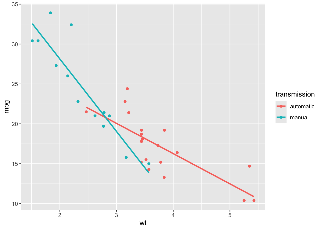

Tip

Use the plot to check you have interpreted the summary output correctly. The absolute gradient is larger for the manual group, and the manual group has a higher intercept.

4.6 Predictions

Given a new observation \(i\) with regressor variables given by a row vector \(\boldsymbol{x}_i^T\) (similar to a row of the design matrix \(X\)), there are two types of interval we may want to construct, a confidence interval for the expected value of the response, \(\boldsymbol{x}_i^T\boldsymbol{\beta}\), and a prediction interval for the value of the response itself. We should expect the prediction interval to be wider as the response has the extra variability coming from the error term in the model.

4.6.1 Confidence interval for the expected value of the response

For estimation of the mean we use the fact that \[\boldsymbol{\hat{\beta}} \sim N_p(\boldsymbol{\beta},\sigma^2(X^TX)^{-1})\] to yield \[\boldsymbol{x}_i^T \boldsymbol{\hat{\beta}} \sim N(\boldsymbol{x}_i^T\boldsymbol{\beta},\sigma^2\boldsymbol{x}_i^T(X^TX)^{-1}\boldsymbol{x}_i)\] so that \[\frac{\boldsymbol{x}_i^T\boldsymbol{\hat{\beta}}-\boldsymbol{x}_i^T\boldsymbol{\beta}}{\sqrt{\sigma^2\boldsymbol{x}_i^T(X^TX)^{-1}\boldsymbol{x}_i}} \sim N(0,1).\]

We cannot calculate the confidence interval from this relationship because we do not know the value of \(\sigma^2\), and we have to replace it with its estimate \(\hat \sigma^2\) and use the \(t\) distribution rather than \(N(0,1)\). Our standardized version of \(\boldsymbol{x}_i^T\boldsymbol{\hat{\beta}}\) becomes \[T=\frac{\boldsymbol{x}_i^T \boldsymbol{\hat{\beta}}-\boldsymbol{x}_i^T \boldsymbol{\beta}}{\sqrt{\hat \sigma^2\boldsymbol{x}_i^T(X^TX)^{-1}\boldsymbol{x}_i}}=\frac{\frac{\boldsymbol{x}_i^T \boldsymbol{\hat{\beta}}-\boldsymbol{x}_i^T \boldsymbol{\beta}}{\sqrt{\sigma^2\boldsymbol{x}_i^T(X^TX)^{-1}\boldsymbol{x}_i}} }{\sqrt{\frac{\hat\sigma^2}{\sigma^2}}},\] and we have \(T \sim t_{n-p}\). Hence a \(100(1-\alpha)\%\) confidence interval for the mean of the predicted value is given by \[\boldsymbol{x}_i^T \boldsymbol{\hat{\beta}}\pm t_{n-p,1-\alpha/2}\sqrt{\hat \sigma^2\boldsymbol{x}_i^T(X^TX)^{-1}\boldsymbol{x}_i}.\]

4.6.2 Prediction intervals for individual observations

A similar argument leads to a \(100(1-\alpha)\%\) prediction interval for the future observation \(y_i\). It is given by \[\boldsymbol{x_i}^T \boldsymbol{ \hat{\beta}}\pm t_{n-p,1-\alpha/2}\sqrt{\hat \sigma^2(1+\boldsymbol{x}_i^T(X^TX)^{-1}\boldsymbol{x}_i)}.\]

The prediction interval for an observation is wider than the confidence interval for the expected value of the observations because of the extra uncertainty coming from the error term (\(\hat \sigma^2\)).

4.6.3 Obtaining and plotting the predictions and intervals in R

Note

To get the predictions and either type of interval, we need to set up a new data frame with the column names for the independent variables the same as those in the original data frame used to fit the model.

For the cars simple linear regression model, we’ll obtain predictions and intervals for 30 values of speed evenly spaced between 1 and 30.

predictDf <- data.frame(speed = 1:30)

We fit the model, assign it to an object, and then use that object in a predict() command. For 95% confidence intervals for the mean response

lmCars <- lm(dist ~ speed, cars)
ciCars <- predict(lmCars, predictDf,
                           interval = "confidence",
                           level = 0.95)
head(ciCars)

         fit        lwr       upr
1 -13.646686 -26.447265 -0.846107
2  -9.714277 -21.733068  2.304513
3  -5.781869 -17.026591  5.462853
4  -1.849460 -12.329543  8.630624
5   2.082949  -7.644150 11.810048
6   6.015358  -2.973341 15.004056

The fit column gives the predictions, and lwr and upr give the confidence interval endpoints.

To get prediction intervals instead, we change the interval argument:

piCars <- predict(lmCars, predictDf,
                           interval = "prediction",
                           level = 0.95)
head(piCars)

         fit       lwr      upr
1 -13.646686 -47.11414 19.82076
2  -9.714277 -42.89057 23.46202
3  -5.781869 -38.68565 27.12192
4  -1.849460 -34.49984 30.80092
5   2.082949 -30.33359 34.49948
6   6.015358 -26.18731 38.21803

Tip

Check the R output makes sense! The predicted values (the fit column) should be the same with either interval = "confidence" or interval = "prediction", but the intervals with the latter argument should be wider.

If we just want to plot confidence intervals for the mean response, we can get this directly with ggplot2: we use the argument se = TRUE in the geom_smooth command:

ggplot(cars, aes(x = speed, y = dist))+
  geom_point()+
  geom_smooth(method = "lm", formula = "y ~ x", se = TRUE)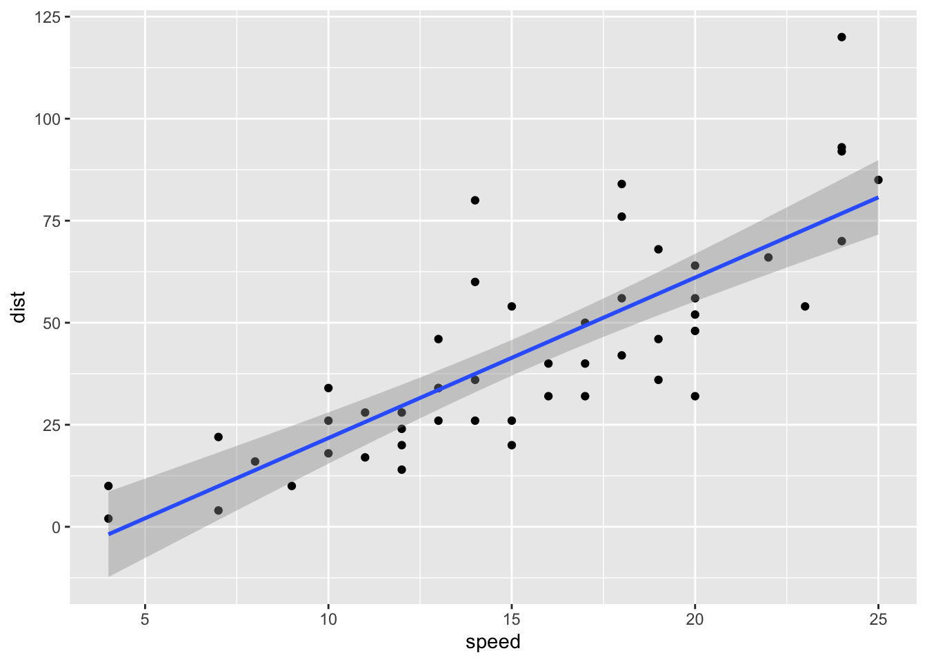

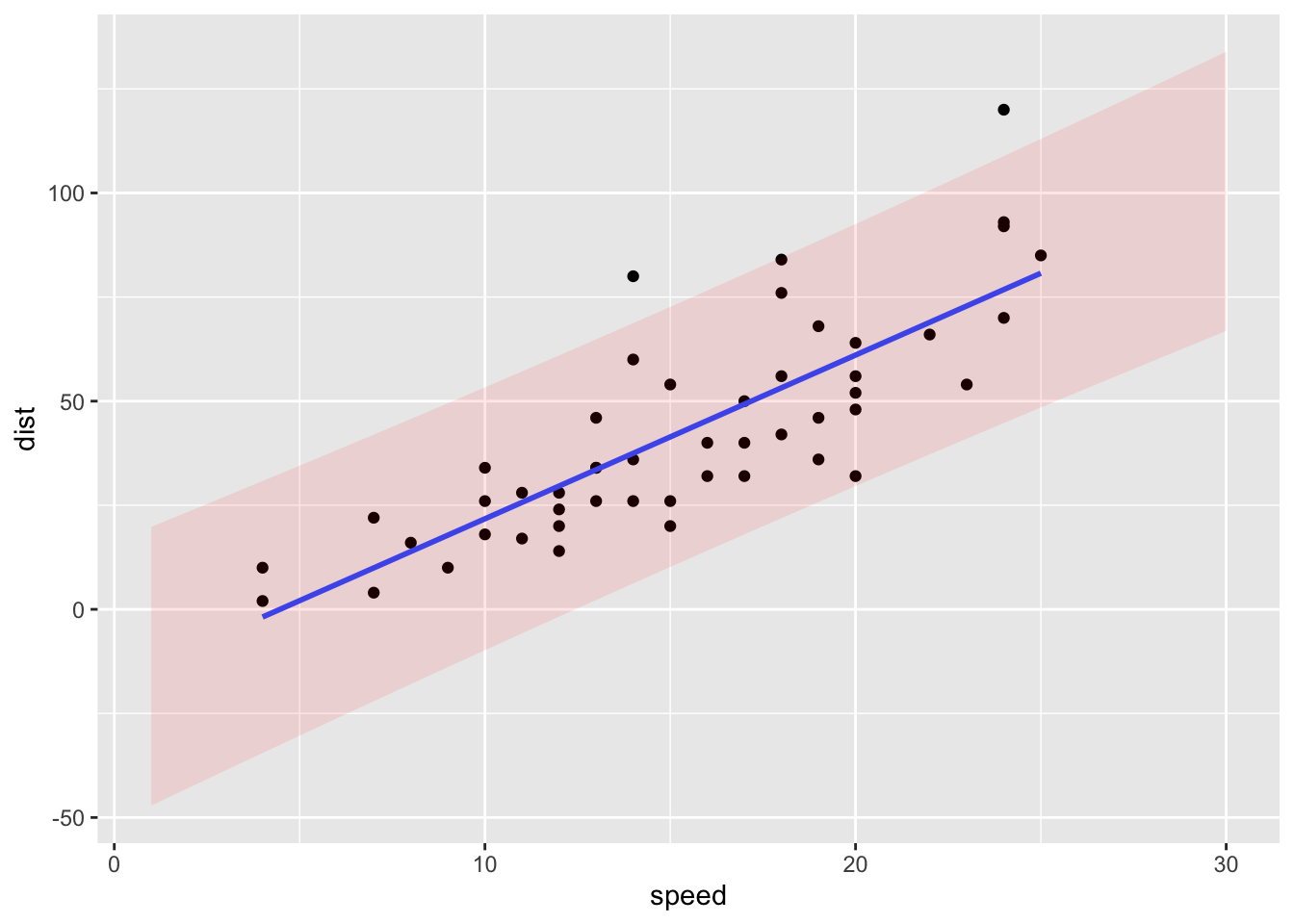
Plotting prediction intervals is more work! Recall that we created prediction intervals and stored them in piCars. We do

ggplot(cars, aes(x = speed, y = dist)) + 
  geom_point() + 
  geom_smooth(method = "lm", formula = y ~ x, se = FALSE) +
  geom_ribbon(data = data.frame(piCars, speed = 1:30),
              aes(x = speed, ymin = lwr, ymax = upr, y = fit),
              alpha = 0.1,
              fill = "red")