Section 9 Monte Carlo methods
We will now give an illustration of using R to solve some problems in probability using simulation (“Monte Carlo” methods). We will introduce one programming concept to help with this: the for loop1.
9.1 The origins of Monte Carlo
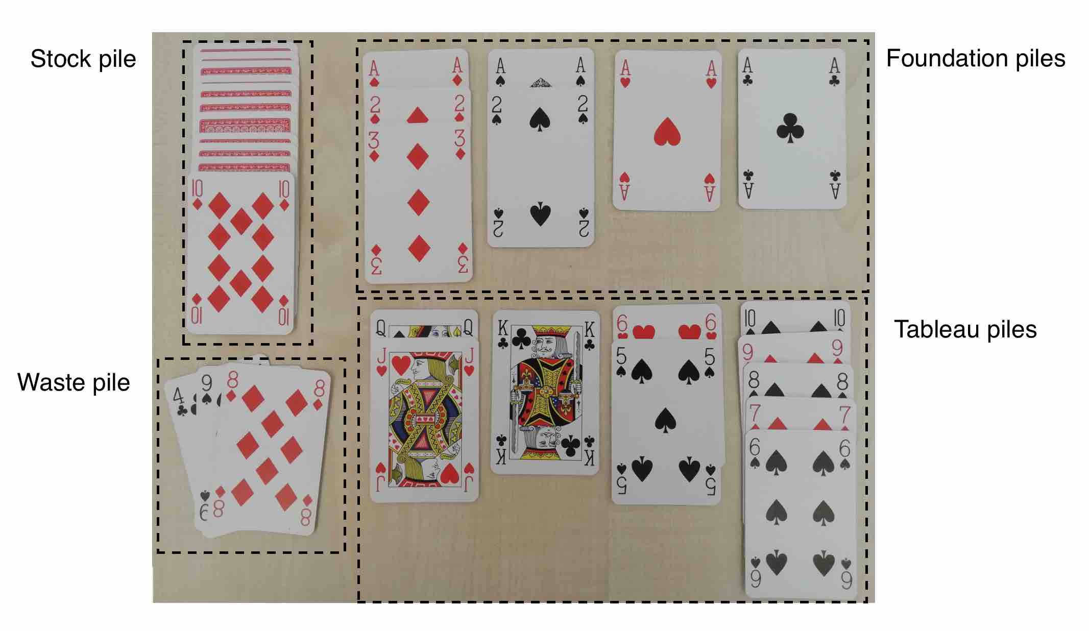
Canfield Solitaire is a card game where you have to arrange all 52 cards into four ‘foundation’ piles, one for each suit, with the cards in increasing order, following rules about when to turn over cards and when to move cards between the various piles. (You don’t actually need to know the rules for this tutorial, and they are quite hard to understand until you’ve seen someone play the game!)
Could you work out the probability of winning the game?
Working this out analytically would be incredibly hard, but there is another way: the Monte Carlo method, invented by the Polish mathematician and physicist Stanislaw Ulam (1909-1984). He wrote2:
“The first thoughts and attempts I made to practice [the Monte Carlo Method] were suggested by a question which occurred to me in 1946 as I was convalescing from an illness and playing solitaires. The question was what are the chances that a Canfield solitaire laid out with 52 cards will come out successfully? After spending a lot of time trying to estimate them by pure combinatorial calculations, I wondered whether a more practical method than”abstract thinking” might not be to lay it out say one hundred times and simply observe and count the number of successful plays. This was already possible to envisage with the beginning of the new era of fast computers, and I immediately thought of problems of neutron diffusion and other questions of mathematical physics, and more generally how to change processes described by certain differential equations into an equivalent form interpretable as a succession of random operations. Later [in 1946], I described the idea to John von Neumann, and we began to plan actual calculations.”
So, we could get an estimate of the probability by
- playing the game lots of times;
- counting the proportion of times we win.
This might still take a long time, but we could instead get a computer to simulate playing the game a large number of times, and then see how many times the computer wins. Using (computer generated) simulations to estimate probabilities (and other quantities) is known as the Monte Carlo method. We can use the Monte Carlo method to get approximate solutions to lots of problems that would be too difficult to solve otherwise.
Programming the Monte Carlo method for the Canfield solitaire problem would be hard, but we can illustrate the method on a simpler example.
9.2 The birthday problem
Suppose there are twenty people in a room. Ignore leap years, and suppose that each person is equally likely to have been born on any day of the year. What is the probability that at least two people in the room have the same birthday?
We can actually solve this problem analytically (which we’ll do later), but it’s a good example for learning about R and the Monte Carlo method. The Monte Carlo method will involve
- getting R to simulate twenty random birthdays;
- determining whether any of the simulated birthdays are the same;
- repeating steps 1 and 2 lots of times, and counting the proportion of times we observe two or more of the twenty random birthdays to be the same.
In the next section, we’ll look at how to use ‘for loops’ as a means of repeating a process multiple times.
for loops are not strictly necessary for these sorts of problems, but they are easy to write and read; it can be easier to understand the link between the mathematical algorithm and its computer implementation.↩︎
Eckhardt, Roger (1987). Stan Ulam, John von Neumann, and the Monte Carlo method. Los Alamos Science (15): 131–137.↩︎