Section 13 R Markdown
R Markdown (Allaire et al. 2020), (Xie, Allaire, and Grolemund 2018) is a system for producing reports. From a single R Markdown document, you can produce your report in a variety of formats including: PDF, Word document, web page (html), slides (including Powerpoint and Beamer).

(Artwork by @allison_horst)
The main idea is that your text and R code go in the same document. When you compile (or “knit”) your document, the R code is run, and the code input and output can be displayed in your report. This has several advantages.
- Your analyses will be more transparent and reproducible. If someone else (or even you at some point in the future) want to know, say, what calculations were done to produce a particular result in the report, the R Markdown document can be inspected to see what R code was used to get the result.
- You will save a lot of time if you need to include plots in your report: you write the code to make your plot, and then R Markdown inserts the plot in your report automatically.
- If changes are made to the data, or if you make some change early on in your analysis, you can just recompile your report, and the code will be re-run with the new data, and all the new results will appear in the re-compiled report. (You may, of course, need to change your text commentary)
13.1 Making html and PDF documents
You can always produce a report in html format. If you want to make PDF documents, you will need LaTeX installed on your computer. If you don’t have LaTeX installed, a suggestion is to install a ‘lightweight’ version TinyTeX, which you can do within R:
Similarly, if you want to make Word documents, you will need Word installed.
13.2 A five minute video tutorial
This video illustrates the basics of how to work with an R Markdown document.
Exercise 13.1 Put your solution to the birthday problem exercise inside an R Markdown document. Include some plain text that briefly explains what probability you are estimating. Produce a histogram of the number of unique birthdays by including the command
Knit your document to html.
13.3 Code chunk options
This video illustrates how to use code chunk options to change the appearance of a document
(One useful option that I didn’t mention in the video is include = FALSE. This will run the code, but will not display the input or any output, including messages and warnings.)
13.3.1 Code chunk options for figures
For reference, here’s an example code chunk with the options you would typically need to use when making a plot. (If you want to run this code, you will need to install the package ggplot2.)
```{r, fig.align = 'center', fig.cap = "My figure caption", fig.height = 3, fig.width = 3}
ggplot2::ggplot(mtcars, ggplot2::aes(x = wt, y = mpg)) +
  ggplot2::geom_point()
```
Some trial and error may be needed to find values for fig.height and fig.width that give the figure size you want.
If importing a figure rather than generating it in R, you may find the option out.width = "60%" easier to work with than fig.height and fig.width. Again, you may need trial and error to decide on the best percentage value.
13.4 Spell checking
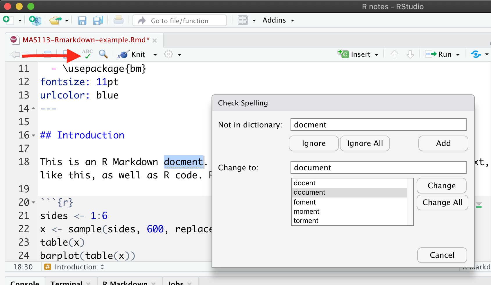
RStudio has a spell checker. To use it, click the green tick (with ABC above) button, in the document window.

If you wish, you can go to Tools > Global Options… > Spelling and change the Main dictionary language to English (United Kingdom).
Using the spell checker will not identify all possible errors. Proofread your work carefully!
Exercise 13.2 Use suitable code chunk options to change the appearance of your R Markdown document from the previous Exercise.
- Make sure no R code appears in your html/pdf document
- Include a figure caption, centre-align your figure, and manually set an appropriate figure size.