Section 14 Probability Distributions in R
We can use R to compute and evaluate all common probability distributions. For each distribution, there are four associated R functions that are identified by the letter prefix at the start of the distribution’s function name as follows:
- ‘d’ denotes the probability density function, pdf (or probability mass function, pmf, for discrete distributions);
- ‘p’ denotes the cumulative distribution function, cdf;
- ‘q’ denotes the quantile function (inverse cdf);
- ‘r’ denotes the function to simulate random draws from the distribution (random generation).
Some key discrete distributions that you will work with include:
| \(\ \ \) | Binomial | Poisson |
|---|---|---|
| pmf | dbinom(\(x\), size, prob) | \(\quad\) dpois(\(x\), lambda) |
| cdf | pbinom(\(q\), size, prob) | \(\quad\) ppois(\(q\), lambda) |
| quantile | qbinom(\(p\), size, prob) | \(\quad\) qpois(\(p\), lambda) |
| random generation | rbinom(\(n\), size, prob) | \(\quad\) rpois(\(n\), lambda) |
and some continuous distributions are:
| \({}\) | Uniform | Exponential | Normal |
|---|---|---|---|
| dunif(\(x\), min, max) | \(\ \ \quad\) dexp(\(x\), rate) | dnorm(\(x\), mean, sd) | |
| cdf | punif(\(q\), min, max) | \(\ \ \quad\) pexp(\(q\), rate) | pnorm(\(q\), mean, sd) |
| quantile | qunif(\(p\), min, max) | \(\ \ \quad\) qexp(\(p\), rate) | qnorm(\(p\), mean, sd) |
| random generation | runif(\(n\), min, max) | \(\ \ \quad\) rexp(\(n\), rate) | rnorm(\(n\), mean, sd) |
14.1 Example
A company claims that, for a particular product, 8 out of 10 people prefer their brand A over a rival’s brand B. We randomly sample 50 people, and ask them whether they prefer brand A to brand B. Let the random variable \(X\) be the number of people who choose brand A. If the company is right, we have that \(X\sim Bin \left(n=50, \ p=\frac{4}{5}\right)\). Using R:
- Calculate the probability that \(X = 40\).
## [1] 0.139819- Calculate the probability that \(X ≤ 30\).
## [1] 0.0009324365- Calculate the value of \(X\) such that 90% of the time, the sampled people will prefer Brand A.
## Here we want to compute the 0.9 quantile (90th percentile) of the probability distribution.
## Hence, we use the quantile function:
qbinom(p = 0.9, size = 50, prob = 0.8)
## [1] 44- Under the company’s assumption, simulate the sample experiment 100 times and plot a histogram of the simulated values for \(X\).
## Under the company's assumption, we use the random generation function to simulate the sample
## given the assumed Binomial distribution 100 times and record the simulated value of X in each case:
X100 <- rbinom(n = 100, size = 50, prob = 0.8)

## plot the histogram of the simulated X values:
hist(X100, xlab = "X", main = "", freq = FALSE)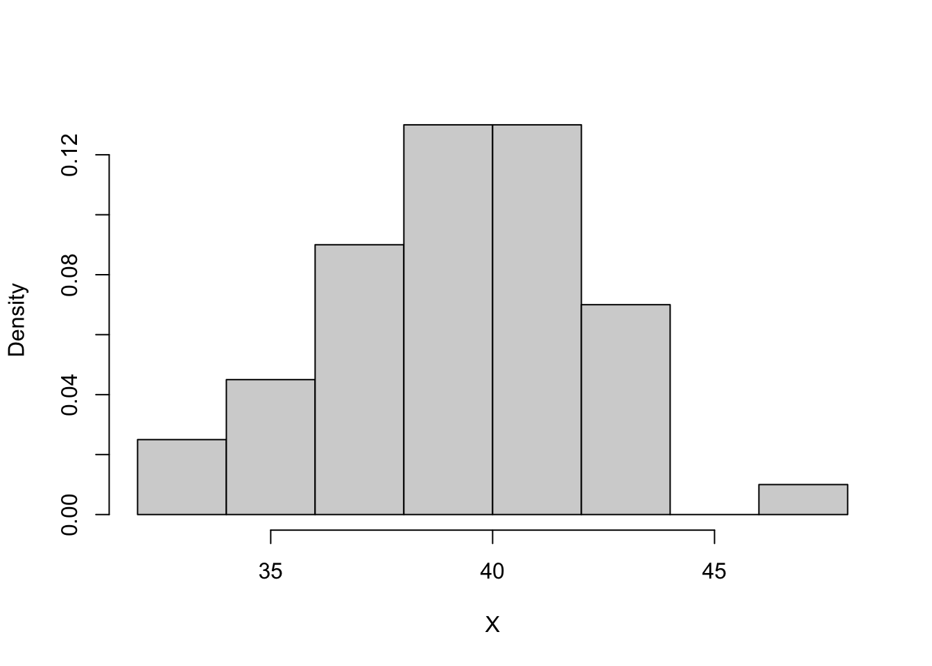
Exercise 14.1
A new pharmacy has opened near a doctors surgery, and over the first week the pharmacist observes an average of 3 customers visiting the pharmacy every 20 mins. Let the random variable \(Y\) represent the number of customer visits in a 20 min period in the following week. Assuming the rate of customer visits remains the same, then we have that \(Y\sim Poisson \left(\lambda = 3\right)\). Using R:
Calculate the probability that in a randomly selected 20 minute period, only 1 customer visits the pharmacy.
Calculate the probability that at least 4 customers will visit in a 20 minute period.
\(~\)
A city zoo holds a large colony of humboldt penguins and the zookeepers have information on the characteristics of the penguins. Letting the random variable \(Z\) represent the weight of a penguin in the colony, they assume that \(Z\) follows a Normal distribution with a mean of 4.4kg and a standard deviation of 0.4kg, i.e. \(Z\sim N \left(4.4, \ 0.4^{2}\right)\). Using R:
Calculate the probability that a randomly selected penguin will weigh less than 4kg.
Estimate the weight that the zookeepers should expect 95% of their colony will not exceed, given the assumption of this distribution.
Create a random sample of 1000 penguin weights using this distribution and plot it as a histogram. Using your sample, compute the probability from part a. and compare your answer. Increase your sample size to 10000. Does the accuracy of your probability estimate improve?