Section 17 Missing data
It is common to find missing values when provided with a data set. In this Section, we’ll briefly discuss how R represents and handles missing data, and some simple options for ‘imputing’ (estimating) missing data, should that be appropriate.
If we come across missing data, it’s important to try to understand why the data are missing. For example, if in some clinical trial, a patient drops out (resulting in missing data) because the treatment wasn’t working, we can’t just delete the patient from our data set for convenience; we’d be be ignoring something important about how effective the treatment is.
17.1 NA
R represents a missing observation with NA. For example, we can create a vector with missing elements as follows,
and we can test to see if there are missing elements with the function is.na():
## [1] FALSE FALSE TRUE FALSE TRUE
If possible, do not remove missing data at the data
cleaning/processing stage. Rather, store the missing values as
NA, so you have a record of them, and then use appropriate
methods to handle missing values inside R.
17.2 Functions and NA
Some functions will, by default, return NA if the vector has any missing elements, e.g.
## [1] NAhowever, there is usually an argument to specify whether to remove missing values, e.g.
## [1] 4Alternatively, the function na.omit() can be used to first remove missing values:
## [1] 4If used with a data frame, na.omit() will exclude rows where any single column has a missing value:
## x y
## 1 2 11
## 2 4 12
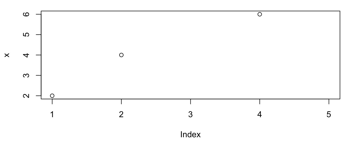
## 4 6 14Plot commands will typically ignore missing values (although you may get a warning message), for example
17.3 Imputation
In some cases, it may be desirable to ‘impute’ (estimate) missing values, and there are different options (and R packages) for doing this. We will briefly illustrate one package, imputeTS (Moritz and Bartz-Beielstein 2017). This package has a nice ‘cheat sheet’ which illustrates its functions.
Suppose we have a vector with some missing values, which we will create as follows, and treat as a time series.
Then, some options for imputing the missing values are
- impute using the mean of all the non-missing cases
##  [1] 0.440000 1.770000 5.768571 5.768571 5.130000 7.720000 7.460000 5.768571
## [9] 8.310000 9.550000- impute using the most recent observed value, “last observation carried forward” (e.g. estimate
x[3]byx[2])
## [1] 0.44 1.77 1.77 1.77 5.13 7.72 7.46 7.46 8.31 9.55- impute using linear interpolation (e.g. linearly interpolate between
x[2]andx[5]to getx[3]andx[4], assuming the observations are uniformly separated in time)
## [1] 0.440 1.770 2.890 4.010 5.130 7.720 7.460 7.885 8.310 9.550- impute using a Kalman smoother (see MAS61005 Time Series)
##  [1] 0.440000 1.770000 2.982747 4.155760 5.130000 7.720000 7.460000 7.985058
##  [9] 8.310000 9.550000
The plot below shows the imputed values (as red circles) in each case.
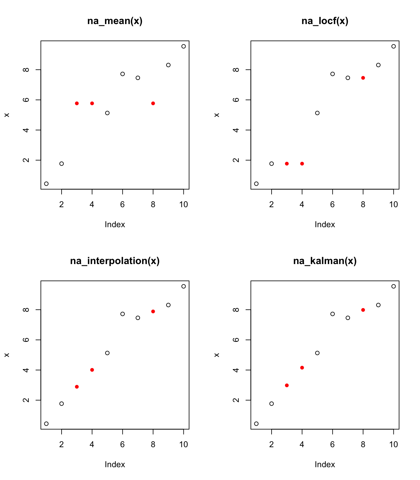
Modelling-based estimates such as those from the Kalman smoother typically involve models in which we observe some process of interest plus noise/measurement error. Estimates obtained from imputation would be of this ‘underlying’ process, not estimates of what would actually be observed.
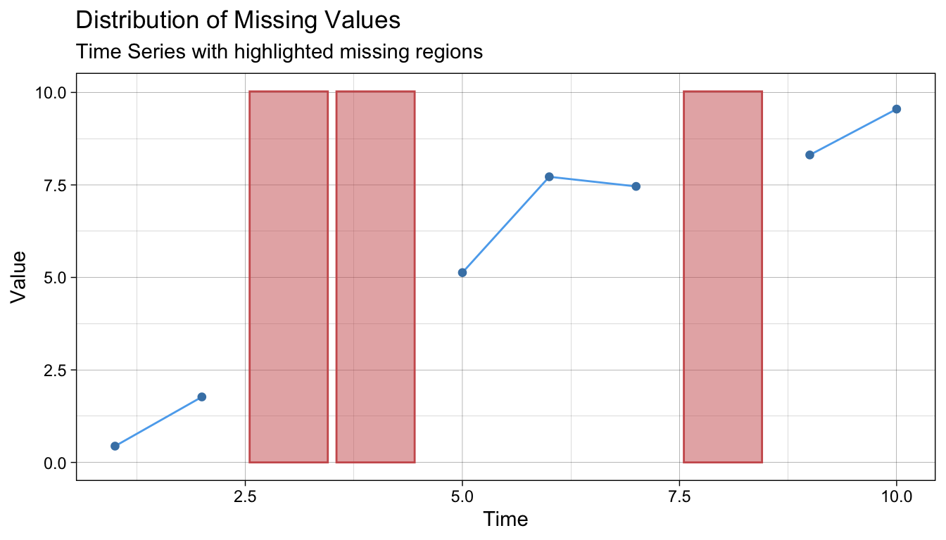
17.4 Visualising missing data
The imputeTS package has some nice plotting functions for missing data. The plots make use of ggplot2 (which we will cover later), but you don’t need to know any ggplot2 syntax to use these functions.
We can produce a plot to show clearly where the missing data are using
 and if we have used imputation, we can make a plot that clearly displays the imputed values with (using
 na_kalman() as an example):

17.5 Exercise
Exercise 17.1 The built-in data frame airquality includes time-series data of four variables, and has missing values in the Ozone and Solar.R variables. Produce plots that indicate where these missing observations are, and plots that show imputed values using the last observed observation for each variable.
17.6 Further reading
CRAN task view on missing data - discussion of various approaches and R packages for handling missing data.
There will be some discussion of missing data in MAS61006 Bayesian Statistics and Computational Methods.