Section 23 Shiny
Shiny (Chang et al. 2020) is an R package for producing apps that can be run from a web-browser. The app will have R running in the background, and so you would either host the app on a suitable server, or you could run the app on your own computer.
You might use a shiny app to make your methods/analyses more accessible to others who don’t use R, or you might find the interactivity that shiny offers a more convenient way of working with R. A gallery of examples is available at https://shiny.rstudio.com/gallery/.
You will need the packages shiny, tidyverse, and MAS6005. The MAS6005 package is on GitHub only (not CRAN); if you haven’t installed it already then use the commands
You will also need the MAS61004Data.zip file. This contains a shiny folder, with the data and some example code.
23.1 Some example R code, for inclusion in an app
We’ll start with some R code to analyse the flint data from the MAS61004Data.zip file. The data are measurements of the length and breadth, in centimetres, of each item in a small group of flint tools, and we suppose there is interest in predicting length given breadth only (e.g. if a tool is damaged). A simple linear regression model will be fitted, with length as the dependent variable, and breadth as the independent variable.
Suppose we want to plot the flint data, together with either a confidence interval for the mean, or a prediction interval for a new observation. Some code is as follows (and is also available in the file flint-script.R).
We will first load in the data
and specify as variables the interval type and level.
Now we’ll compute the desired interval and put everything together in a new data frame.
lmFlint <- lm(length ~ breadth, flintDf)
intervalDf <- cbind(flintDf,
                predict(lmFlint,
                        interval = intervalType,
                        level = cpLevel))
Note that we’ve made use of the previously defined variables cplevel and intervalType in the predict() command.
Now we’ll draw the plot
ggplot(intervalDf, aes(x = breadth, y = length)) +
  labs(x="flint tool breadth (cm)", y="flint tool length (cm)") +
  geom_point() +
  geom_line(aes(y = fit)) +
  geom_ribbon(aes(ymin = lwr, ymax = upr),
              fill = "red", alpha = 0.1) +
ylim(3, 6.5) 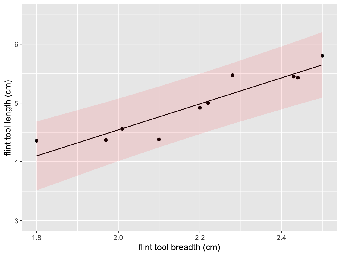
We’ll also produce a correlation matrix, firstly defining the type of correlation we want
and then using this variable inside a further command:
##           breadth    length
## breadth 1.0000000 0.9294603
## length  0.9294603 1.0000000
Now suppose we want to try a different type/size of interval, or a different correlation method. We would redefine our variables cpLevel, intervalType and/or corMethod, for example, to be
and run the rest of the code again. This may not be very convenient, and if we wanted a ‘client’ to be able to make such changes; he/she would have to know how to use R.
23.2 Putting the code inside an app
We’re now going to create a shiny app, where the user can change the three variables cpLevel, intervalType and corMethod at any time. Whenever one of these variables is changed, the new plot or correlation will be displayed as appropriate.
A shiny app has two components: a user interface ui, where the controls are specified and the outputs are arranged, and a server, where all the R computation is done. The structure of the code will look like something like this:
ui <- fluidPage(# controls and outputs to be specified here
  )

server <- function(input, output) {
  # computations to be done here
}

# Run the application
shinyApp(ui = ui, server = server)
Open the file flint-app-simple.R and click on Run App to run the app. Try it out, have a look at the code, and then continue below for discussion of how the app works. (You will need to close the app before you can use the R console again.)
23.3 The user interface ui
A user interface can have three types of commands: specifying user controls, producing outputs, and modifying the layout/appearance of the app.
Commands within ui need to end in a comma, unless they
are either the final command in ui, or they are the final
command nested within another command
This takes a little getting used to, and can be a common source of bugs in shiny apps! Look carefully again at flint-app-simple.R.
23.3.1 Commands (“widgets”) for creating user controls and inputs
In our example, we had three variables that we wanted to change easily: cpLevel, intervalType, corMethod. In the app, within the user interface ui, we define a widget where the app user can specify the value of a variable. There are lots of different types of widgets, depending on the type of variable the user is specifying (e.g. numerical or string).
For example, to allow the app user to define the cpLevel variable, we define a numericInput widget inside the ui definition:
numericInput(inputId = "cpLevel",
                label = "Interval level (%)",
                min = 0, max = 100,
                value = 95,
step = 1)- The variable name is the
inputIDargument.
To use a variable created in ui in the
server, we must add the prefix input$. So,
for example, to use the variable cpLevel in the
server, we must refer to it as
input$cpLevel.
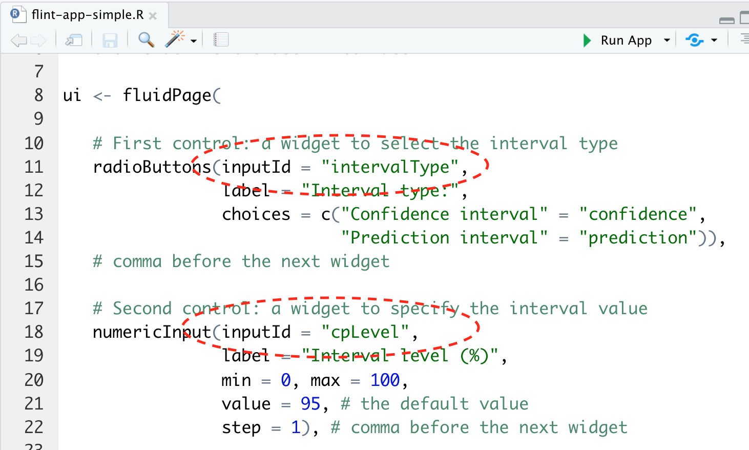
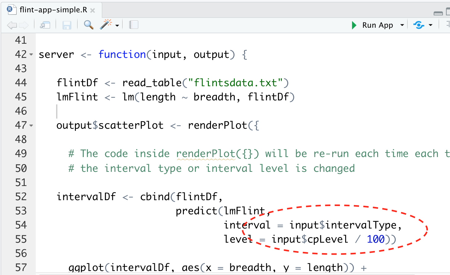
Figure 23.1: The top image shows part of the ui definition, in which the variables intervalType and cpLevel are defined via the widgets radioButtons and numericInput. The bottom image shows the use of these variables in the server definition. Note the input$ prefix: the variables are referred to as input$intervalType and input$cpLevel.
- In the app interface, the variable will be described by the text in
label. - We can also specify a minimum (
min), maximum (max), a default value (value), and a step size (step) for increasing/decreasing the variable if clicking on arrows.
In the example flint-app-simple.R, we used two other widgets, radioButtons(), and selectInput() to define intervalType and corMethod respectively.
The widget gallery at RStudio is a good place to see examples of more widgets.
23.3.2 Commands for producing outputs
An output is typically a plot, a table, or a single numerical value. In our example app, we want a plot and a table (correlation matrix), which we produce with these commands plotOutput() and tableOutput() inside our definition of ui.
We choose scatterPlot and correlations as labels for use inside server.
Commands can also be added for determining the layout and appearance of the app; we haven’t used any of these yet, but will add some in later on.
23.4 The server
Here, we put the commands to do the computation and make the various outputs we have declared in our user interface; the commands that will actually draw a plot, for example.
Firstly, we put the commands for loading the data and fitting the model inside server:
These could have gone in the script (before server is defined), but not inside the definition of ui. (In some situations, you will need to think carefully about where exactly commands are placed, but we don’t need to worry about this now.)
23.4.1 Making a plot
Firstly, recall that in our ui definition, we had the code
so, inside server, we will need to create something called output$scatterPlot, defined with a function renderPlot({}) to make this plot.
All our earlier code for making the plot can go inside the renderPlot({}), with one modification: we now refer to the variables cpLevel and intervalType with the syntax input$cpLevel and input$intervalType:
output$scatterPlot <- renderPlot({
  intervalDf <- cbind(flintDf,
                      predict(lmFlint,
                              interval = input$intervalType,
                              level = input$cpLevel / 100))

  ggplot(intervalDf, aes(x = breadth, y = length)) +
    labs(x = "flint tool breadth (cm)",
         y = "flint tool length (cm)") +
    geom_line(aes(y = fit)) +
    geom_point() +
    geom_ribbon(aes(ymin = lwr, ymax = upr),
                   fill = "red", alpha = 0.1) +
    ylim(3, 6.5)
})23.5 Reactivity
An important concept to understand, that (within R) is particular to shiny is that of reactivity: this is where the magic happens! How does R know it should redraw the plot/table when an input changes? In the shiny version of the code, cpLevel, intervalType and corMethod are all specially defined as reactive variables. This means that shiny is on the look-out for when these variables change their values: it will know that the current plot/table are ‘invalid’, and need redrawing, using the updated values.
- Reactive variables can also be defined within the
server, but we won’t cover this here. - We have to be careful where we try to call a reactive variable: shiny will complain if we try to call one outside a ‘reactive context’. For example, if we move the definition
outside the output$scatterPlot <- renderPlot({}) definition, we will get an error message (try putting the command straight after the definition of lmFlint).
Exercise 23.1 Open the script medals-script.R, and first run the code to produce
- a plot of total medals against population size with either a raw or log 10 transformed \(x\)-axis;
- a medals table, either ranked by number of gold, or number of golds divided by the country’s population size.
Now produce an app where the user can switch between axis type and medal ranking format, with an option of how many countries are displayed in the table. You will probably find it easiest to make a copy of flint-app.R and modify that.
23.6 Customising the appearance of your app
You can include various commands in ui to change the appearance of your app. A few useful ones are as follows
titlePanel()for adding a title;sidebarPanel()andmainPanel()for having the widgets displayed on the left side, and the outputs shown in the right;tabsetPanel()andtabPanel()for splitting up multiple outputs into different tabs.
Commands will need to be nested, and you have to be even more careful where to put the commas! Open up the file flint-app-modified.R and run the app to see some examples (and look carefully to see where the commas go!)
Exercise 23.2
Try modifying your Olympic medals app to include a title, a sidebar and main panel, and tabs.
23.7 Shiny with R Markdown
You can embed a Shiny app inside an R Markdown (html) document. If you want to include text, static images and so on, this may be more convenient that incorporating these directly in the app with html commands.
You just need to add an extra argument in the YAML header, and then Shiny commands will work:
---
title: "My shiny app"
author: "Jeremy Oakley"
output: html_document
runtime: shiny
---
For an example, see the file flint-app-document.Rmd.
23.8 Further reading
This section has covered the main ideas you will need for this module (though you may want to try out other widgets). There are some excellent materials for further study available at https://shiny.rstudio.com/tutorial/. In particular some topics for suggested reading/viewing are as follows.
- shiny modules. If you are designing a more complex app, the length of your code may become awkward to manage and/or you may want to repeated use of the same elements within an app. shiny modules can be useful here.
- Generating downloadable reports. A disadvantage of using a shiny app is that it can be hard to record how you used it: what values you gave to the inputs and so on. One option is to use R markdown to generate a report for downloading, making use of the input values currently selected in the app.
- Automated testing. How to test whether your app does what it is supposed to, and if you make changes, how to you check that you haven’t accidentally broken your app.
- Reactivity (and also part 2) If you really want to get your head around reactivity, I recommend these two videos, that include programming exercises. You will need to be comfortable with the shiny basics.
- Online textbook: Mastering Shiny A print copy is also available.
- More on shiny in R Markdown documents from Chapter 19 of R Markdown: The Definitive Guide.