Section 21 R Markdown
R Markdown (Allaire et al. 2020), (Xie, Allaire, and Grolemund 2018) is a system for producing reports. From a single R Markdown document, you can produce your report in a variety of formats including: PDF, Word document, web page (html), slides (including Powerpoint and Beamer).
 (Artwork by @allison_horst)
The main idea is that your text and R code go in the same document. When you compile (or “knit”) your document, the R code is run, and the code input and output can be displayed in your report. This has several advantages.
- Your analyses will be more transparent and reproducible. If someone else (or even you at some point in the future) want to know, say, what calculations were done to produce a particular result in the report, the R Markdown document can be inspected to see what R code was used to get the result.
- You will save a lot of time if you need to include plots in your report: you write the code to make your plot, and then R Markdown inserts the plot in your report automatically.
- If changes are made to the data, or if you make some change early on in your analysis, you can just recompile your report, and the code will be re-run with the new data, and all the new results will appear in the re-compiled report. (You may, of course, need to change your text commentary)
21.1 A five minute video tutorial
This video illustrates the basics of how to work with an R Markdown document.
21.2 Working directories for R Markdown documents
When we run a code chunk inside an R Markdown document, the working directory is set to be directory containing the document (check this by running the command getwd() inside a code chunk.) If you are using an RStudio project, you may wish your data and R Markdown documents to be in different folders, e.g., if the project directory is myProject, you may have folders
myProject/data
myProject/reports
If your R Markdown document is in the folder myProject/reports, and you want to import a file myData.csv from myProject/data, specify the (relative) file path in your R Markdown document as
Exercise 21.1 Create an R Markdown document that presents some of your solutions to the exercises in Section 18.7 on the Brexit data.
You may need to install RMarkdown first, using the command
- For now, make a document that presents one plot only.
- Knit your document to html.
- If you have LaTeX on your computer, try knitting to pdf as well.
- The goal of this exercise is simply to produce a working document: do not worry about how your document looks. You will change the appearance of your document in later exercises.
21.3 Code chunk options
This video illustrates how to use code chunk options to change the appearance of a document
(One useful option that I didn’t mention in the video is include = FALSE. This will run the code, but will not display the input or any output, including messages and warnings.)
21.3.1 Code chunk options for figures
For reference, here’s an example code chunk with the options you would typically need to use when making a plot.
```{r, fig.align = 'center', fig.cap = "My figure caption", fig.height = 3, fig.width = 3}
ggplot(mtcars, aes(x = wt, y = mpg)) +
  geom_point()
```
Some trial and error may be needed to find values for fig.height and fig.width that give the figure size you want.
If importing a figure rather than generating it in R, you may find the option out.width = "60%" easier to work with than fig.height and fig.width. Again, you may need trial and error to decide on the best percentage value.
Exercise 21.2 Use suitable code chunk options to change the appearance of your R Markdown document from the previous exercise.
- Make sure no R code appears in your html/pdf document
- Include a figure caption, centre-align your figure, and manually set an appropriate figure size.
21.4 Tables
There are several options for producing tables in R Markdown. (For general advice on formatting tables, see Section 22.3 of Wilke (2019).
21.4.1 Using Markdown
Here’s an example of making a table with the Markdown syntax. Note the use of : for specifying text alignment.
| column 1 | column 2 | column 3 |
|:---------|:--------:|---------:|
| left     | centre   | right    |
| aligned  | aligned  | aligned  |
This is rendered as follows.
| column 1 | column 2 | column 3 |
|---|---|---|
| this text | this text | this text |
| is left | is centre | is right |
| aligned | aligned | aligned |
Online tools are available for generating Markdown syntax, for example https://www.tablesgenerator.com/markdown_tables.
21.4.2 Using knitr::kable()
The knitr package (Xie 2020b), (Xie 2014), (Xie 2015) has the kable() function which can produce a table from a data frame. Here’s an example.
which is rendered (in html) as follows:
| mpg | cyl | disp | hp | drat | wt | qsec | vs | am | gear | carb | |
|---|---|---|---|---|---|---|---|---|---|---|---|
| Mazda RX4 | 21.0 | 6 | 160 | 110 | 3.90 | 2.620 | 16.46 | 0 | 1 | 4 | 4 |
| Mazda RX4 Wag | 21.0 | 6 | 160 | 110 | 3.90 | 2.875 | 17.02 | 0 | 1 | 4 | 4 |
| Datsun 710 | 22.8 | 4 | 108 | 93 | 3.85 | 2.320 | 18.61 | 1 | 1 | 4 | 1 |
| Hornet 4 Drive | 21.4 | 6 | 258 | 110 | 3.08 | 3.215 | 19.44 | 1 | 0 | 3 | 1 |
| Hornet Sportabout | 18.7 | 8 | 360 | 175 | 3.15 | 3.440 | 17.02 | 0 | 0 | 3 | 2 |
| Valiant | 18.1 | 6 | 225 | 105 | 2.76 | 3.460 | 20.22 | 1 | 0 | 3 | 1 |
21.5 Caching results for slow-running code
If some of your code takes a long time to run, it is preferable not to re-run it every time you edit your R Markdown document and want to re-compile it. It you use the code chunk option cache = TRUE, R will store (‘cache’) the results, and will only re-run the code chunk if it detects that something has changed.
Be careful if you use caching. For example, if you import a file and cache the results, R will not detect if the file contents change. When you knit your final version of your document, switch off all caching.
Exercise 21.3 Add one table to your R Markdown document from the previous exercise, to show the mean percentage of the remain vote grouped by area. Use knitr::kable() to produce the table.
21.6 Spell checking
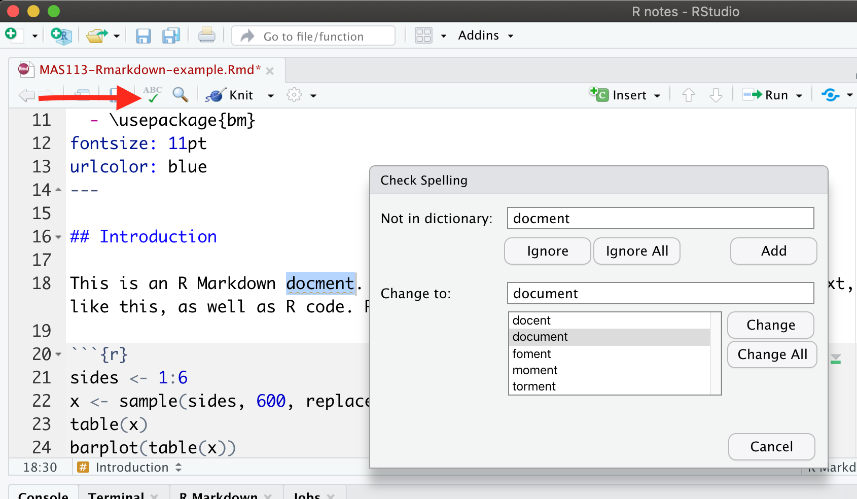
RStudio has a spell checker. To use it, click the green tick (with ABC above) button, in the document window.
If you wish, you can go to Tools > Global Options… > Spelling and change the Main dictionary language to English (United Kingdom).
Using the spell checker will not identify all possible errors. Proofread your work carefully!
21.7 The YAML header
The first part of an R Markdown document, the ‘header’ is used to specify information such as author and title, and can include extra commands to change the appearance of the document. These are commands are specified using another language called YAML. Here’s an example of a YAML header, with a few extra commands specified that you might find helpful.
---
title: "My Report Title"
author: "Jeremy Oakley"
date: "2024-09-03"
output:
  pdf_document:
    number_sections: true
  html_document:
    number_sections: true
fontsize: 11pt
urlcolor: blue
header-includes:
  - \usepackage{bm}
---
Indenting of particular lines does matter in YAML. Keep this is mind when copying YAML examples.
The command Sys.Date() is an R command which will insert today’s date (year-month-day format). The commands fontsize and urlcolor affect pdf output only. The final command
header-includes:
  - \usepackage{bm}
can be used to add commands (e.g. \usepackage{bm}) to the preamble in the LaTeX document for pdf output.
21.8 LaTeX, Markdown and html
The Markdown language is broadly the same as LaTeX for typesetting equations/maths notation, and so you can use LaTeX as normal for typesetting maths.
You can use any other LaTeX commands throughout your document. When producing pdf output, R Markdown will actually generate an intermediate .tex file, which is then compiled to pdf. However, these commands will be ignored if you knit to html or other formats.
Similarly, you can include html commands in your document; these will only work if you knit to html.
Try to keep to Markdown commands as far as possible. This will give you the most flexibility regarding your choice of output format (and you may wish to switch your output format in the future.)
For example, putting this in your document:
\section{Introduction}will only produce the desired section heading if you knit to pdf, but using this:
# Introductionwill give the desired section heading for any output format you produce.
21.9 bookdown
bookdown (Xie 2020a), (Xie 2017) is an extension to R Markdown, that has extra features helpful for writing books, dissertations and longer reports/articles. (I used bookdown to produce this ‘gitbook’ that you are reading now.) You won’t need bookdown on this module, but we will provide a template and instructions for your dissertation.
Exercise 21.4 Using your document from the previous exercise:
- edit the YAML header to increase the font size for pdf output
- add a short amount of text to explain the subject of your document;
- use RStudio’s spell checker.
21.10 Quarto
Quarto is a newer system for producing documents, and is described by its authors as “the next generation of R Markdown”. Quarto is designed to work with a greater variety of languages and platforms; it can be used without an installation of R.
If you use Quarto within RStudio, you will find it very similar to using R Markdown, and Quarto will render most .Rmd files without modification.
R Markdown will be sufficient for this module, but you can use Quarto if you wish. For more details, see the Quarto homepage.