Chapter 6 Hypothesis testing: A-level recap

This chapter recaps the basic ideas in hypothesis testing that are covered at A-level (though we will not assume that you have studied hypothesis testing before). In the next few chapters we will cover some further hypothesis testing problems, as well as studying a general simulation approach, which will give you more insight into how hypothesis testing works.

In a hypothesis test, we make some assumption (the “hypothesis”) about the distribution of the data, typically specifying the values of the parameters of the distribution, and then test whether the data ‘contradict’ this assumption.

There are two general approaches to hypothesis testing, which are very similar, but differ in how the conclusions are reported. We will refer to these as Neyman-Pearson testing, and Fisher’s p-value method³.

6.1 Hypothesis testing with the Neyman-Pearson approach

Suppose a company is developing a vegetarian substitute for minced beef, and is aiming for a product which is indistinguishable from meat. The substitute is to be tested in an experiment. Fifty volunteers will be each be given two portions of lasagna: one made with beef, and one with the vegetarian substitute, and asked to identify which lasagna is meat-free. The company will analyse the results of the experiment with a hypothesis test, and will make a decision about whether to continue with their product based on the results.

This is a scenario in which Neyman-Pearson testing could be used. The general procedure is as follows.

Choose an appropriate statistical model and hypotheses

Define $X$ to be the number of people who correctly identify the meat-free lasagna. We might suppose that \[ X\sim Bin(50, \theta) \] If the substitute is indistinguishable from minced beef, the volunteers would, in effect, be guessing with a probability of 0.5 of guessing correctly. Suitable null and alternative hypotheses would then be \[\begin{align} H_0 &: \theta = 0.5 \quad \mbox{(null hypothesis),}\\ H_A &: \theta \neq 0.5\quad \mbox{(two-sided alternative hypothesis).} \end{align}\]

Choose the size or significance level of the test

When stating the conclusion of the test, we will either state we “reject $H_0$” (conclude that $H_0$ is false), or we “do not reject $H_0$” (and then carry on as if $H_0$ is true). There are two ways, therefore, in which we could make the wrong conclusion. These are referred to as type I and type II errors.

Definition 6.1 (Type I error) A Type I error is the mistake of rejecting the null hypothesis when the null hypothesis is actually true.

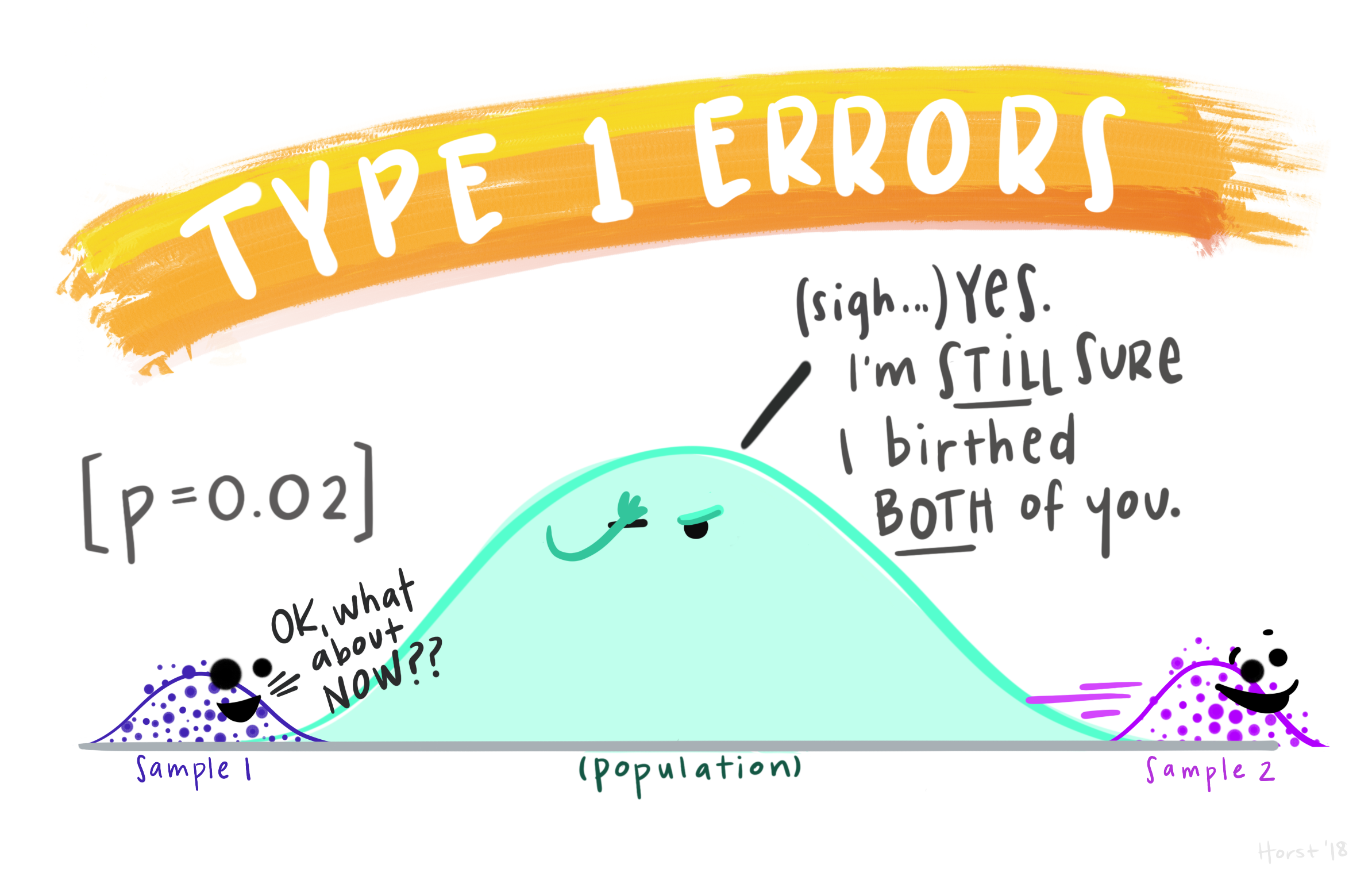
$A type I error: falsely rejecting $H_0$. We think we have discovered something ‘interesting’ in our data, but have been deceived by random variation. Artwork by @allison_horst.$

Figure 6.1: A type I error: falsely rejecting $H_0$. We think we have discovered something ‘interesting’ in our data, but have been deceived by random variation. Artwork by @allison_horst.

Definition 6.2 (Type II error) A Type II error is the mistake of failing to reject the null hypothesis when the null hypothesis is actually false.

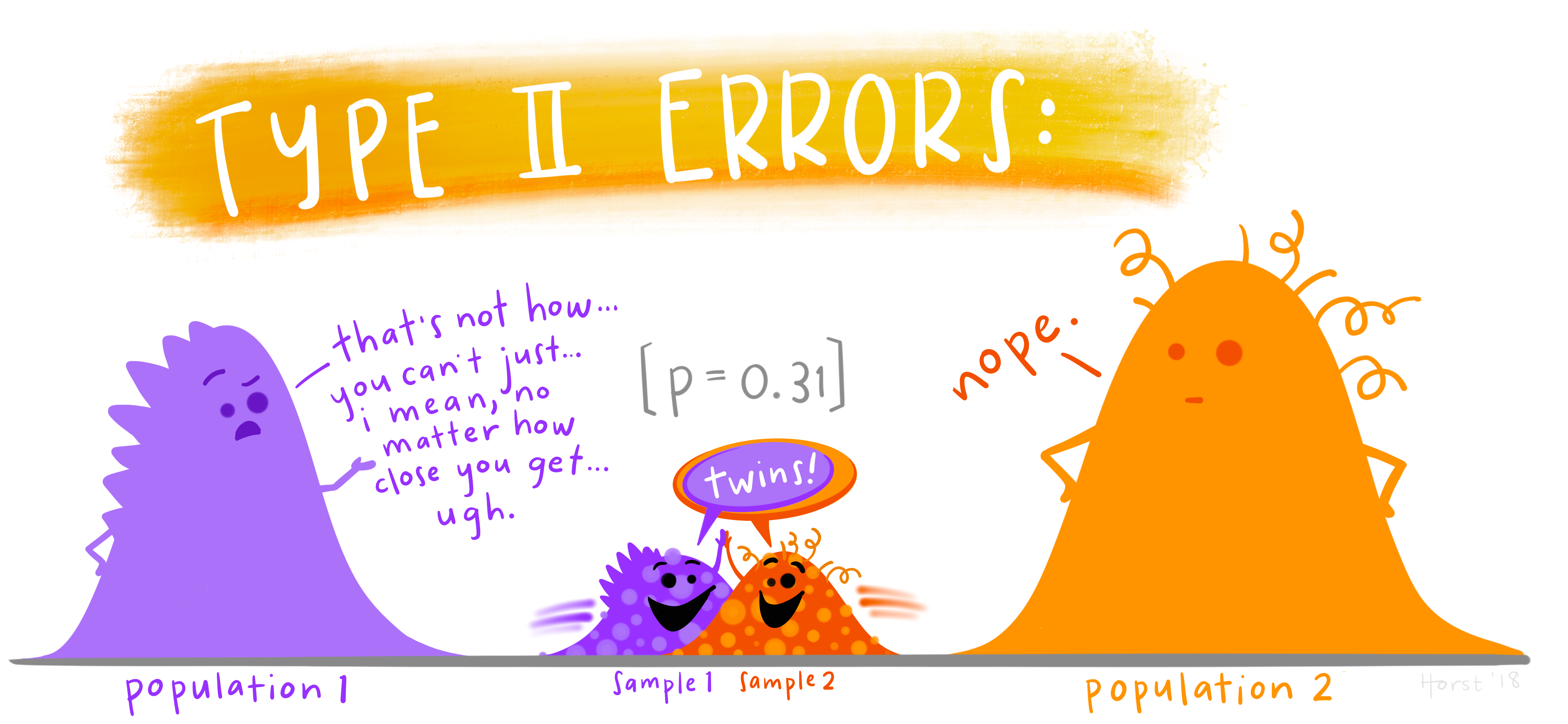
$A type II error: failing to reject $H_0$ when $H_0$ is really false. Here, random variation has hidden a potentially interesting discovery. This can result from having too small a sample size. Artwork by @allison_horst.$

Figure 6.2: A type II error: failing to reject $H_0$ when $H_0$ is really false. Here, random variation has hidden a potentially interesting discovery. This can result from having too small a sample size. Artwork by @allison_horst.

Definition 6.3 (Size / level of significance) The size of a test is the probability, before we get our data, that we would make a Type I error. The size of a test is also known as the level of significance. The size/level of significance is often denoted by $\alpha$.

In Neyman-Pearson testing we choose, in advance, the size of test. A common choice of size/significance level is 5%, so the probability of a Type I error would be 0.05. Why not choose 0%, so that a Type I error is impossible? The only way to make Type I errors impossible is to refuse ever to reject the null hypothesis, but this then increases the risk of a Type II error; we have to trade off risks of the two error types. Choosing a small value such as 5% is a compromise.

Choose a test statistic

A test statistic measures ‘how different’ the data are from what we would expect under $H_0$.

In our example, we use the test statistic \[\begin{equation} Z = \frac{\frac{X}{n} - \theta_0}{\sqrt{\theta_0(1-\theta_0)/n}}, \end{equation}\] with $n$ the sample size, and $\theta_0$ the hypothesised values of $\theta$ under $H_0$ (so in the example, we have $n=50$ and $\theta_0=0.5$). This measures how far the observed proportion of correct responses is from $\theta_0$ (the proportion we’d expect if $H_0$ were true), scaled by the standard deviation of $X/n$ (again, if $H_0$ were true).

We’d expect (the absolute value of) a test statistic to be small if $H_0$ is true, and to be relatively large if $H_A$ is true.

Identify the critical region

We now find a critical region $C$ such that

a value of $Z$ in the critical region would correspond to a large difference between $X/n$ and $\theta_0$;
the probability of $Z$ falling in the critical region, if $H_0$ were true, would be 0.05 (the size/significance level).

Using the normal approximation to the binomial distribution, we suppose that $Z\sim N(0,1)$ and so the critical region is $(-\infty, -1.96] \cup [1.96, \infty)$

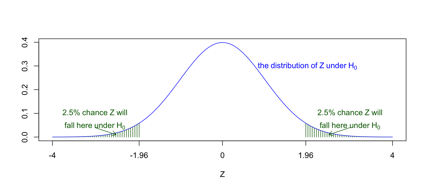
$The distribution of the test statistic assuming $H_0$ is true, and the 5% critical region shaded in green. There is only a 5% chance of the test statistic falling in this region if $H_0$ is true: we will reject $H_0$ if the test statistic falls in this region.$

Figure 6.3: The distribution of the test statistic assuming $H_0$ is true, and the 5% critical region shaded in green. There is only a 5% chance of the test statistic falling in this region if $H_0$ is true: we will reject $H_0$ if the test statistic falls in this region.

Compute the test statistic for the observed data, and state the conclusion

If the observed value of $Z$ falls in the critical region, we declare that we reject $H_0$ (at the 5% level of significance); otherwise, we declare that we do not reject $H_0$. For example, if 40 out of 50 people correctly identified the meat-free lasagna, the observed test statistic, denoted by $z_{obs}$ would be \[ z_{obs} = \frac{\frac{40}{50}-0.5}{\sqrt{0.5\times(1 - 0.5) / 50}} = 4.24, \] which does lie in the critical region, so $H_0$ would be rejected. The company may then decide that their substitute hasn’t achieved the taste they want, and they may try something else.

6.1.1 One-sided and two-sided alternative hypotheses

We used an alternative hypothesis

\[ H_A: \theta \neq 0.5. \] This is two-sided because we would want to reject $H_0:\theta = 0.5$ if either $\theta > 0.5$ or $\theta<0.5$. One-sided alternative hypotheses would be \[ H_A: \theta > 0.5, \] or \[ H_A: \theta < 0.5. \] In some situations, it may appear that a one-sided alternative hypothesis is more suitable, e.g. $H_0:$ “the drug has no effect on blood pressure, on average” and $H_A:$ “the drug lowers blood pressure, on average” (if the aim of the drug was to lower blood pressure). However, there is an argument in this situation for always using a two-sided alternative.

If the drug had the opposite effect to that desired, we would still want to know.
Using a one-sided alternative makes the critical region larger in the area of interest; $H_0$ can be rejected with a smaller observed effect of the drug.

6.2 Fisher’s $p$-value method

In the Neyman-Pearson approach to hypothesis testing, the conclusion is stated in terms of “reject $H_0$”, or “do not reject $H_0$”. We would use this where there is a clear decision to be made after the test. Sometimes, however, we are just interested in whether data supports a particular hypothesis or not; there is no decision or action that follows the test.

A hypothesis test can not prove whether a hypothesis or not. Rather than declaring whether a hypothesis been “rejected”, it might be preferable instead to report the strength of evidence provided by an experiment.

Consider again the example of the vegetarian minced-beef substitute. Suppose the product is already on the market, and a consumer TV show does the same experiment to see if people if can taste the difference. There is no ‘decision’ to be made afterwards; the experiment is done out of public interest.

We have the same model and hypotheses as before. Defining $X$ to be the number of people (out of 50) correctly identifying the vegetarian substitute, we suppose $X\sim Bin(50, \theta)$, with

\[\begin{align} H_0 &: \theta = 0.5,\\ H_A &: \theta \neq 0.5, \end{align}\] so that under $H_0$, people are just guessing. Now consider three scenarios:

Scenario	Data	Test Statistic
A	32 people out of 50 guess correctly	2.06
B	31 people out of 50 guess correctly	1.75
C	40 people out of 50 guess correctly	5.30

If we were using Neyman-Pearson with a test of size 0.05, the critical region for the test statistic would be $(-\infty, -1.96]\cup [1.96, \infty)$; the test statistics would lie in the 5% critical region in scenarios A and C, but not in scenario B.

Comparing scenarios A and B, the results were the nearly the same: only one more person correctly identified the meat substitute in scenario A. Should we really be drawing different conclusions in these two scenarios?
Comparing scenarios A and C, the evidence seems more persuasive in scenario C. Shouldn’t we report this somehow?

In Fisher’s $p$-value method, instead of declaring whether $H_0$ is reject or not, we describe the strength of the evidence against $H_0$, by reporting the $p$-value.

The $p$-value is a probability and, informally, describes how ‘surprising’ the observed data are, assuming $H_0$ to be true.

If the $p$-value is small, it means the data are not what we would expect to see under $H_0$. The smaller the $p$-value, the stronger the evidence against $H_0$.
If the $p$-value is large, the data are consistent with what we’d expect under $H_0$ (but this is not the same as saying we have evidence in favour of $H_0$ being true).

Definition 6.4 ($p$-value) For a test statistic $T$, with observed value $t_{obs}$ and a two-sided alternative hypothesis, we define the $p$-value as \[\begin{equation} P(|T|\ge |t_{obs}|), \end{equation}\] calculated for the distribution of $T$ under $H_0$.

Continuing the example, our test statistic is denoted by $Z$, assumed to have a $N(0,1)$ distribution if $H_0$ is true. The $p$-values in the three scenarios would be:

\[\begin{align*} \mbox {Scenario A:}&\quad P(Z\le -2.06) + P(Z\ge 2.06) \simeq 0.04,\\ \mbox {Scenario B:}&\quad P(Z\le -1.75) + P(Z\ge 1.75) \simeq 0.08,\\ \mbox {Scenario C:}&\quad P(Z\le -5.30) + P(Z\ge 5.30) \simeq 1.2\times 10^{-7}.\\ \end{align*}\]

Note that the $p$-value is much smaller in Scenario C than in A: the evidence against $H_0$ is stronger.

We obtain the numerical probabilities using R, noting that for $Z\sim N(0,1)$, we have $P(Z\le -x) + P(Z\ge x) = 2P(Z\le -x)$. For example

2 * pnorm(-2.06)

## [1] 0.0394

The $p$-value is much smaller in Scenario C, compared with A, and so we can say that the evidence against $H_0$ is much stronger in Scenario C. We visualise the $p$-value in Scenario A below.

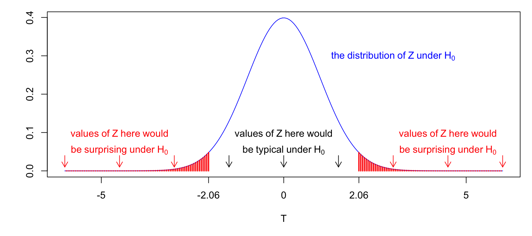
The observed test statistic was 2.06. Is this a suprising value of $Z$ under $H_0$? We report how surprising this value is in terms of how likely we are to get an (absolute) value as large as 2.06, assuming $H_0$ to be true. This is the $p$-value, and is represented by the red shaded area.

Figure 6.4: The observed test statistic was 2.06. Is this a suprising value of $Z$ under $H_0$? We report how surprising this value is in terms of how likely we are to get an (absolute) value as large as 2.06, assuming $H_0$ to be true. This is the $p$-value, and is represented by the red shaded area.

6.2.1 What counts as a small $p$-value?

This varies between scientific fields. In medical research, a $p$-value of 0.05 or smaller would typically count as ‘significant’ evidence against the null hypothesis. If a scientist wants to claim a new discovery, and publish the results of his/her experiment in an academic journal, some journals will require a $p$-value less than 0.05 for the article to be published, although one journal banned this practice⁴. Particle physicists are rather more demanding! They require a $p$-value smaller than 0.003 for “evidence of a particle”, and smaller than 0.0000003 for a “discovery”⁵.

For this module we will use the following convention

$p$-value	Interpretation
$p > 0.05$	No evidence against $H_0$
$0.05 \ge p > 0.01$	Weak evidence against $H_0$
$0.01 \ge p > 0.001$	Strong evidence against $H_0$
$0.001 \ge p$	Very strong evidence against $H_0$

In particular, for $p$-values just below 0.05, a recommendation would be to repeat the experiment to look for confirmation.

6.3 Relationship between the Neyman-Pearson and $p$-value methods

Note that if the $p$-value is less than 0.05, we can deduce that the test statistic must lie in the 5% critical region. Hence some people use a combination of both methods, and say things like, “The $p$-value is less than 0.05, so we have statistically significant evidence against $H_0$ at the 5% level.” Reporting the $p$-value gives a little more information: we are saying how strong the evidence is against $H_0$, and not simply whether $H_0$ is rejected or not. We illustrate this in Figure 6.5.

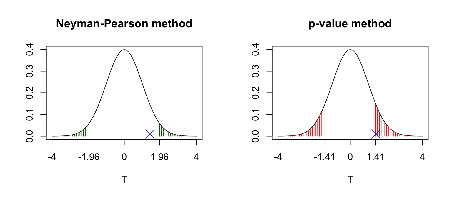
$Suppose our observed test statistic was 1.41, as shown by the blue cross. For the Neyman-Pearson method, with a test of size 0.05, we determine the critical region which has a 5% chance of containing the test statistic $T$, assuming $H_0$ is true. This is shown as the green shaded area; this area is 0.05. For the $p$-value method, we calculate the probability that $T$ would be as or more extreme as our observed test statistic $t_{obs}$, assuming $H_0$ is true. This is shown as the red shaded area. If the $p$-value (red shaded area) is greater than 0.05, we can deduce that the test statistic $t_{obs}$ cannot lie in the 5% critical region.$

Figure 6.5: Suppose our observed test statistic was 1.41, as shown by the blue cross. For the Neyman-Pearson method, with a test of size 0.05, we determine the critical region which has a 5% chance of containing the test statistic $T$, assuming $H_0$ is true. This is shown as the green shaded area; this area is 0.05. For the $p$-value method, we calculate the probability that $T$ would be as or more extreme as our observed test statistic $t_{obs}$, assuming $H_0$ is true. This is shown as the red shaded area. If the $p$-value (red shaded area) is greater than 0.05, we can deduce that the test statistic $t_{obs}$ cannot lie in the 5% critical region.

6.4 Which hypothesis test do I use for…?

There are a large number of hypothesis tests covering a range of situations. Over the next few chapters we will consider three (studying more than this would be tedious!):

comparing two means;
comparing two proportions;
analysing contingency table data.

You will see that the general approach is the same in each case. All that change are

the test statistic that is computed;
the distribution of the test statistic under the null hypothesis.

Once you have understood how things work in general, you should be confident in tackling any hypothesis testing problem: search for the problem online (or in a textbook), identify the choice of test statistic and its distribution under $H_0$, and then you should find the implementation straightforward.

devised by the statisticians Jerzy Neyman (1894-1981), Egon Pearson (1895-1980) and Sir Ronald Fisher (1890-1962).↩︎
https://www.statslife.org.uk/news/2116-academic-journal-bans-p-value-significance-test ↩︎
https://blogs.scientificamerican.com/observations/five-sigmawhats-that/↩︎

\(p\)-value	Interpretation
\(p > 0.05\)	No evidence against \(H_0\)
\(0.05 \ge p > 0.01\)	Weak evidence against \(H_0\)
\(0.01 \ge p > 0.001\)	Strong evidence against \(H_0\)
\(0.001 \ge p\)	Very strong evidence against \(H_0\)

An Introduction to Data Science

Chapter 6 Hypothesis testing: A-level recap

6.1 Hypothesis testing with the Neyman-Pearson approach

6.1.1 One-sided and two-sided alternative hypotheses

6.2 Fisher’s \(p\)-value method

6.2.1 What counts as a small \(p\)-value?

6.3 Relationship between the Neyman-Pearson and \(p\)-value methods

6.4 Which hypothesis test do I use for…?