Chapter 8 Hypothesis testing: comparing two proportions

In this chapter we will test whether the probability parameters $\theta_X$ and $\theta_Y$ in two binomial distributions $X\sim Bin(n, \theta_X)$ and $Y\sim Bin(m, \theta_Y)$, are equal or not, given observations from each distribution. In particular, when might we conclude that $\theta_X$ and $\theta_Y$ are different, based on an observed difference between $X/n$ and $Y/m$?

We will again use two different methods: a computer simulation method, and an analytical method based on the normal distribution.

8.1 Example: an investigation into gender bias

Steinpreis et al. (1999)⁹ conducted the following experiment. CVs were sent to male and female academic psychologists at various US universities. The psychologists were asked whether or not they would hire the applicant for an academic job based on the CV. The CVs sent to the psychologists were identical except for the name of the applicant: “Brian Miller” on some, and “Karen Miller” on the others. The interest was in whether the gender of the applicant made a difference: whether male applicants were more or less likely to be hired than female applicants.

Results from the experiment were as follows. The “recruiters” are the academic psychologists. There are 128 different recruiters: each recruiter sees one CV only, where the applicant is either male or female.

applicant	recruiter	hired	rejected	% hired
male	male	24	7	77.4%
female	male	16	16	50.0%
male	female	22	10	68.8%
female	female	13	20	39.4%

The data suggest a clear gender bias: male applicants are more likely to be hired (regardless of the gender of the recruiter). But can we be sure of this? We’d expect recruiters to have different opinions anyway, and we can see that within each row of the table, some recruiters must have been more demanding of their applicants than others, in that some chose to hire, and others chose to reject. Perhaps we were just unlucky with our sample of recruiters? For example, perhaps in row two of the table, recruiters tended to be more demanding than the recruiters in row one? We can investigate this using a hypothesis test (as did the study authors, though they used a slightly different method.)

8.2 Comparing two binomial proportions

To simplify things, we’ll just consider the male recruiters:

applicant	recruiter	hired	rejected	% hired
male	male	24	7	77.4%
female	male	16	16	50.0%

The observed difference in % hired for the two groups was 27.4% Could a difference this large arise purely by chance?

We use a binomial model for the data, with a separate binomial distribution for the number of recruiters choosing to hire in each row of the table: defining $X$ as the number of recruiters who would hire the male applicant, and $Y$ as the number of recruiters who would hire the female applicant, we suppose that

\[\begin{align} X &\sim Binomial(n, \theta_X),\\ Y &\sim Binomial(m, \theta_Y), \end{align}\] with $n = 31$ and $m=32$. We interpret $\theta_X$ and $\theta_Y$ as, respectively, the proportion of all recruiters in the population who would hire the male applicant, and the proportion of all recruiters in the population who would hire the female applicant.

If the gender of the applicant was irrelevant to all recruiters, then we would have $\theta_X = \theta_Y$, and we will write our null hypothesis as \[ H_0: \theta_X = \theta_Y. \]

8.2.1 A simulation method

As before, we need to understand what sort of data could arise purely by chance. In our gender bias example, we need to understand how different $X/n$ and $Y/m$ could be, if $H_0$ were true and the probabilities $\theta_X$ and $\theta_Y$ were the same.

In the experiment, the observed values of $X$ and $Y$ were 24 and 16 (with the observed difference in proportions being $\frac{24}{31} - \frac{16}{32}\simeq 27\%$).

If it’s (almost) impossible to get a difference this large purely by random chance, we would conclude that the experiment has provided evidence against the hypothesis that the two probabilities $\theta_X$ and $\theta_Y$ are equal.
If it’s easy to get a difference this large purely by random chance, we won’t say this shows $H_0$ is true, but we will say that the experiment has failed to provide evidence against $H_0$.

Let’s now see what can happen purely by chance, using simulation. We will need to choose $\theta_X$ and $\theta_Y$, which we need to be equal if we are assuming $H_0$ is true. We’ll choose these probabilities to equal the total number of hires (40) divided by the total number of recruiters (63).

We’ll first simulate five $X,Y$ pairs in R: we simulate five observations from the $Binomial(31, 40/63)$ distribution, and store the result in the vector males and five observations from the $Binomial(32, 40/63)$ distribution, and store the result in the vector females:

males <- rbinom(n = 5, size = 31, prob = 40/63)
females <- rbinom(n = 5, size = 32, prob = 40/63)

Then to see what we’ve got:

males

## [1] 21 21 19 16 22

females

## [1] 17 16 19 19 24

and to compare the proportions:

males/31 - females/32

## [1]  0.14617  0.17742  0.01915 -0.07762 -0.04032

The first pair generated for $(X,Y)$ was (21, 17), and the difference between the two proportions was $\frac{21}{31} - \frac{17}{32} \simeq 0.15$: we got a 15% difference in the proportions hired, just by random chance. However, we didn’t get anything as large as the observed difference of 27%. Now we will do this a large number of times, and look at the distribution of the difference between the proportions:

males <- rbinom(n = 100000, size = 31, prob = 40/63)
females <- rbinom(n = 100000, size = 32, prob = 40/63)
differences <- males/31 - females/32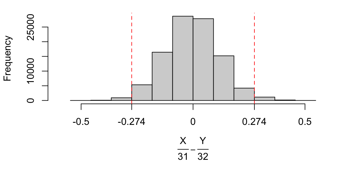

Histogram of simulated differences $X/31 - Y/32$, randomly generated assuming $H_0$ is true. It is possible to obtain differences larger than 0.274 (the difference observed in the experiment), but not very likely; it's hard to obtain a difference this large by random chance alone.

Figure 8.1: Histogram of simulated differences $X/31 - Y/32$, randomly generated assuming $H_0$ is true. It is possible to obtain differences larger than 0.274 (the difference observed in the experiment), but not very likely; it’s hard to obtain a difference this large by random chance alone.

We can see that it is possible to get a difference as large as 0.274, but not that likely. Out of the 100,000 simulations, we can count how many times this happened:

sum(differences >= 0.274)

## [1] 1306

so we would estimate the probability of seeing a difference as large as 0.274, purely by random chance, to be 1306 $/$ 100000 $\simeq$ 0.013.

What about the negative differences, in particular those, below -0.274? Should we count those? This depends on whether we want to report

how far apart $X/n$ and $Y/m$ could be, purely by random chance, or
how much greater $X/n$ could be than $Y/m$, purely by random chance.

In this case, a large negative value of $X/n-Y/m$ would still suggest unequal treatment of males and females, so we should report the first case above. This means that we are using a two-sided alternative hypothesis

\[ H_A: \theta_X \neq \theta_Y, \] rather than a one-sided alternative $H_A: \theta_X> \theta_Y$.

So we calculate how many times we generated obtained $|X/31 - Y/32|\ge 0.274$ (use the abs() command in R to get the absolute value)

sum(abs(differences) >= 0.274)

## [1] 2308

So in conclusion, we report the value of

\[ P\left(\left|\frac{X}{31} - \frac{Y}{32}\right|\ge 0.274\right), \] assuming $H_0$ to be true, which we estimate to be 100000.274 $/$ 100000 $\simeq$ 0.023.

In summary:

we estimate about a 2% probability that, by nothing other than random chance, the (absolute) difference in percentages of hired applicants between the genders could be as large as 27.4% (the difference that was observed in the experiment).

This probability of 2% is a $p$-value: a probability of getting a difference as extreme as the one we observed, assuming $H_0$ to be true.

8.3 An analytical method

So we can write this in general terms, we will define $x$ and $y$ as the observed values of the random variables $X$ and $Y$ (in the example, we have $x=21$ and $y=17$). We used simulation to estimate \[ P\left(\left|\frac{X}{n} - \frac{Y}{m}\right|\ge \left|\frac{x}{n} - \frac{y}{m} \right|\right), \] assuming $H_0$ to be true. We will now attempt to work out this probability analytically, by expressing it in terms of a standard probability distribution. We have

\[ P\left(\left|\frac{X}{n} - \frac{Y}{m}\right|\ge \left|\frac{x}{n} - \frac{y}{m} \right|\right) = P\left(\frac{\left|\frac{X}{n} - \frac{Y}{m}\right|}{\sqrt{v}}\ge\frac{ \left|\frac{x}{n} - \frac{y}{m} \right|}{\sqrt{v}}\right) \]

where we define \[ v:= p^*(1-p^*)\left(\frac{1}{n} + \frac{1}{m}\right) \] with \[ p^*: = \frac{x+y}{n+m} \] Now we define \[ Z:= \frac{\frac{X}{n} - \frac{Y}{m}}{\sqrt{v}} \] If we assume $H_0$ is true, and we further assume $\theta_X = \theta_Y = \frac{x+y}{n+m}$ (just as we did to simulate our random data), then we have

\[\begin{align} \mathbb{E}(Z) &= 0,\\ Var(Z)&=1. \end{align}\] (Deriving these results is an exercise in the tutorial questions.)

We now make the approximation that $Z\sim N(0,1)$ (using the result that a $Binomial(n,p)$ distribution can be approximated by a $N(np, np(1-p))$ distribution, for ‘large’ $n$ and ‘moderate’ $p$.).

We didn’t have to make any approximations about normal distributions in the simulation method, so we can think of that as more ‘accurate’ than this analytical method. But maybe we’ll get similar results! We will soon see…

To compute the $p$-value, we can write

\[\begin{align} P\left(\left|\frac{X}{n} - \frac{Y}{m}\right|\ge \left|\frac{x}{n} - \frac{y}{m} \right|\right)&= P\left(|Z| \ge \frac{\left|\frac{x}{n} - \frac{y}{m} \right|}{\sqrt{v}}\right)\\ & P\left(Z \le - \frac{\left|\frac{x}{n} - \frac{y}{m} \right|}{\sqrt{v}}\right) + P \left(Z\ge \frac{\left|\frac{x}{n} - \frac{y}{m} \right|}{\sqrt{v}}\right)\\ &\simeq \Phi\left(-\frac{\left|\frac{x}{n} - \frac{y}{m} \right|}{\sqrt{v}}\right) + 1 - \Phi \left(\frac{\left|\frac{x}{n} - \frac{y}{m} \right|}{\sqrt{v}}\right ), \end{align}\] where $\Phi(.)$ is the cumulative distribution function of the $N(0,1)$ distribution.

In our example, with $n=31, m=32, x = 24, y = 16$, we compute

\[p^* =\frac{24 + 16}{31 + 32},\quad v = p^*(1-p^*)\left(\frac{1}{31}+ \frac{1}{32}\right) \] and our p-value is \[ \Phi(-2.2599) + 1 - \Phi(2.2599)= 0.024, \] to 3 d.p. Notice how similar this is to the $p$-value computed using simulation. We visualise the $p$-value in Figure 8.2, where we plot the distribution of $Z$ under $H_0$. For comparison, we also plot the histogram of our simulated values $X/31 - Y/32$, each now divided by $\sqrt{v}$.

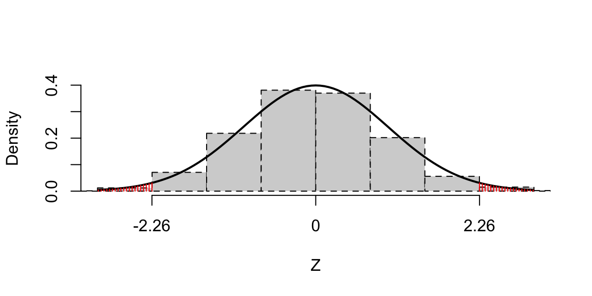
The distribution of the test statistic $Z$ under $H_0$. For comparison, a histogram shows the distribution of test statistics obtained using random simulation: note the close agreement.

Figure 8.2: The distribution of the test statistic $Z$ under $H_0$. For comparison, a histogram shows the distribution of test statistics obtained using random simulation: note the close agreement.

8.3.1 The analytical method: a summary

To summarise, the steps are as follows.

State the model and hypotheses

We wish to compare two binomial proportions. We have

\[ X\sim Bin(n,\theta_X), \] \[ Y\sim Bin(m,\theta_Y) \] and our null hypothesis is \[ H_0:\theta_X = \theta_Y, \] the ‘success’ probabilities in our two samples are the same. For a two-sided alternative, we have \[ H_A: \theta_X \neq \theta_Y \]

Choose an appropriate test statistic

The test statistic measures the difference between the two sample proportions. We use use the test statistic \[\begin{equation} Z = \frac{\frac{X}{n} - \frac{Y}{m} }{\sqrt{P^*(1-P^*)\left(\frac{1}{n}+\frac{1}{m}\right)}}, \end{equation}\] where \[\begin{equation} P^* = \frac{X+Y}{n+m} \end{equation}\]

State the distribution of the test statistic, under the assumption that $H_0$ is true

We think of $Z$ as a random variable, because it is a function of the two binomial random variables $X$ and $Y$. If $H_0$ is true, then approximately, we have \[Z\sim N(0,1).\]

Calculate the test statistic for the observed data

Remembering that we denote the values we actually observed by $x$ and $y$, the corresponding observed value of the test statistic is

\[ z_{obs} = \frac{\frac{x}{n} - \frac{y}{m} }{\sqrt{p^*(1-p^*)\left(\frac{1}{n}+\frac{1}{m}\right)}}, \] where \[ p^* = \frac{x+y}{n+m}. \]

Report the evidence against the null hypothesis, by calculating the $p$-value

We have the same definition of the $p$-value as before, but now using the test statistic $Z$ and its corresponding distribution under $H_0$: \[ P(|Z|\ge |z_{obs}|), \]

8.3.2 Conclusion

In statistical terms, we would say that with a $p$-value between 0.01 and 0.05, we have ‘weak’ evidence against the null hypothesis. Given such a $p$-value (and noting that the experiment was fairly small in any case), it would be desirable to replicate the experiment, to see if the results are the same. This has indeed happened: see for example Moss-Racusin et al. (2012)¹⁰], who conducted a similar study, and observed a similar bias against female job applicants.

8.4 Confidence intervals to measure the difference

An approximate 95% confidence interval for the difference $\theta_X - \theta_Y$ is given by \[\begin{equation} \frac{x}{n} - \frac{y}{m} \pm 1.96 \sqrt{v}, \end{equation}\] with \[v = p^*(1-p^*)\left(\frac{1}{n}+ \frac{1}{m}\right),\quad p^* =\frac{x + y}{n + m}. \] In our example, we obtain a 95% confidence interval of (3.6%, 51.2%): this is wide in this context, reflecting a lot of uncertainty.

Example 8.1 (Hypothesis testing: comparing binomial proportions. Can early release and tagging of prisoners affect the likelihood of reoffending?)
Meuer and Woessner (2018)¹¹ describe an experiment to test the effect of electronic monitoring (tagging) on “low-risk” prisoners. We describe some of their data here. Forty-eight (male) prisoners were randomly allocated to two groups:

in the experimental group, the prisoner served the last part of his sentence under “supervised early work release”, involving the use of an open prison and electronic tagging.
in the control group, the prisoner served the last part of his sentence in prison, as normal.

Following the end of the sentence, the prisoners were followed up for two years. It was recorded whether each prisoner reoffended. The results were as follows.

group	sample size	number reoffending	% reoffending
experimental	24	7	29.2%
control	30	15	50.0%

Specify an appropriate model for these data and hypothesis to test.
Use the following R output to assess whether there is evidence that early work release/tagging scheme has affected the probability of reoffending

experimental <- rbinom(n = 100000, size = 24, prob = 22 / 54)
control <- rbinom(n = 100000, size = 30, prob = 22 / 54)
differences <- experimental / 24 - control / 30
sum(abs(differences) >= abs(7/24 - 15/30))

## [1] 13026

Conduct a suitable hypothesis test using the normal approximation. Draw a sketch that indicates the $p$-value. Based on the output above, what do you think the $p$-value would be?
Calculate a 95% confidence interval for the difference between the two probabilities of reoffending.

Solution

Define the random variables $X$ and $Y$ as the numbers reoffending in the experimental and control groups respectively. We suppose

\[ X\sim Bin(24, \theta_X), \quad Y\sim Bin(30, \theta_Y),. \] and our hypotheses are \[ H_0: \theta_X = \theta_Y, \quad H_A: \theta_X \neq \theta_Y. \] 2. The observed difference in proportion was \[ \frac{7}{24} - \frac{15}{30} = -0.208, \] (to 3 d.p.). In the R code, we have simulated $X, Y$ pairs assuming $H_0$ is true, with $\theta_X = \theta_Y =\frac{7 + 15}{24 + 30}$. The last line counts how many times we simulated a pair where the (absolute) difference in proportions was at least 0.208. This happened 13026 times out of 100,000, so we estimate that there is 13% probability of observing, purely by random chance, a difference as large at that seen in the experiment. This probability is relatively high, giving no evidence against $H_0$: no evidence that the early work release/tagging scheme has affected the probability of reoffending.

We compute

\[ z_{obs} = \frac{\frac{7}{24} - \frac{15}{30} }{\sqrt{p^*(1-p^*)\left(\frac{1}{24}+\frac{1}{30}\right)}} = -1.54 , \] (with $p^* = (7+15)/(24+30)$)

The $p$-value is obtained from \[ P(|Z|\ge 1.54), \]

where $Z\sim N(0,1)$, and is shown as the shaded area in the following plot.

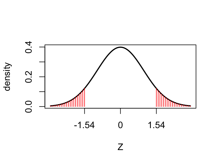from the R output in part (2), we would expect this to be around 0.13. We can obtain the $p$-value from R as follows.

2 * pnorm(-1.54)

## [1] 0.1236

An approximate 95% confidence interval for the difference in proportions is

\[ -0.208 \pm 1.96 \sqrt{v}, \] with $v = p^*(1-p^*)(1/24 + 1/30)$ and $p^* = (7 + 15)/(24+30)$, which gives \[ (-47\%,\,5.5\% ) \]

Steinpreis, R. E., Anders, K. A. and Rizke, D. (1999). The Impact of Gender on the Review of the Curricula Vitae of Job Applicants and Tenure Candidates: A National Empirical Study. Sex Roles, Vol. 41, Nos. 7/8.↩︎
Faculty’s subtle gender biases favor male students, Corinne A. Moss-Racusin, John F. Dovidio, Victoria L. Brescoll, Mark J. Graham, Jo Handelsman, Proceedings of the National Academy of Sciences Sep 2012, 201211286; DOI: 10.1073/pnas.1211286109↩︎
Meuer, K. and Woessner, G. (2018). Does electronic monitoring as a means of release preparation reduce subsequent recidivism? A randomized controlled trial in Germany. European Journal of Criminology, 1-22.↩︎