Chapter 7 Hypothesis testing: comparing two population means
In this chapter we will use hypothesis testing to compare two populations and see if they have different population means. We will use two different methods: a computer simulation method, and an analytical method known as the two-sample \(t\)-test.
7.1 Example: can imagining eating food make you eat less?
Morewedge et al. (2010)6 conducted an experiment to test whether imagining eating food can make one eat less, when offered the same food item to eat. The experiment was repeated by Camerer et al. (2018)7, and we use their data here.
96 student volunteers were recruited, and split into two groups:
In the control group, the participants were each shown a picture of a bowl filled with thirty-three 20-cent coins. They were asked to imagine inserting the coins, one at a time, into a parking meter.
In the treatment group, the participants were each shown a picture of a bowl filled with three 20-cent coins. They were asked to imagine inserting the coins, one at a time, into a parking meter. They were then shown a picture a bowl containing 30 M&Ms, and they were asked to imagine eating the M&Ms, one at a time.
All the participants were then given an actual bowl of M&Ms to eat (containing 40g in total). They were told they were doing a taste test, and were told to eat as much or a little they liked.
Each participant did the experiment in a private cubicle, so no-one watched them eat, but the amount eaten was recorded once they had finished.
Histograms of the amounts eaten for the two groups are shown in Figure 7.1
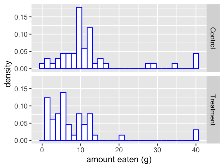
Figure 7.1: Histograms showing the amount of chocolate eaten in each group. The treatment group had to first imagine eating chocolate, before they were given anything to eat. Did it make them want to eat less?
7.1.1 The hypotheses
We define \(\mu_X\) to be the population mean quantity eaten that would be eaten under the control conditions (not imagining eating M&Ms), and \(\mu_Y\) to be the population mean quantity eaten that would be eaten under the treatment conditions (imagining eating M&Ms). The null hypothesis is that imagining eating M&Ms has no effect on consumption:
\[ H_0: \mu_X = \mu_Y \] We choose a two-sided alternative \[ H_A: \mu_X \neq \mu_Y \] as we would be interested if imagining eating M&Ms either resulted in the participants eating more, or eating less on average.
We define:
- \(x_1,\ldots,x_n\): the \(n\) control group observations, with sample mean \(\bar{x}\) and sample variance \(s^2_X\);
- \(y_1,\ldots,y_m\): the \(m\) treatment group observations, with sample mean \(\bar{y}\) and sample variance \(s^2_Y\).
In this example, we have \(n=49\) and \(m=47\).
7.1.2 A test statistic
We measure the difference in mean consumption with the test statistic
\[t_{obs} = \frac{\bar{x} - \bar{y}}{\sqrt{\frac{s^2_X}{n} + \frac{s^2_Y}{m}}}\] so that we scale the difference in means by how much variation there is in the amounts the individuals ate.
In R, the observations are stored in the vectors control and treatment, and we compute \(t_{obs}\) as follows
(mean(control) - mean (treatment))/
  sqrt(var(control)/49 + var(treatment)/47)
## [1] 2.398(We will round this to 2.4 from now on.)
7.2 Hypothesis testing using simulation
All hypothesis testing problems involve understanding what sort of data could arise purely by chance, where “purely by chance” is described by the null hypothesis. In the current example, could the difference in mean consumption have arisen purely by chance?
We will first use a computer simulation technique to investigate this. Let’s look at the first few observations in the treatment group
treatment[1:4]## [1] 12 7 5 8We see that person 1 ate 12g, person 2 ate 7g and so on. Suppose the null hypothesis is true, and treatment has no effect. We might then suppose that, had person 1 been allocated to the control group instead, it would have made no difference to how much person 1 ate: he/she would still have eaten 12g. So maybe the difference is purely because more ‘hungry’ volunteers were randomly allocated to the control group than the treatment group.
Could this have happened by chance? We can investigate this as follows, bearing in mind that the randomness we are investigating here is the random allocation of volunteers to groups, and how that could produce unequal mean consumption.
- We first combine all the treatment and control observations into a single vector called
everyone.
everyone <- c(treatment, control)so to see all the observations:
everyone## [1] 12 7 5 8 40 4 4 11 7 5 13 11 10 4 7 2 13 12 2 2 9 10 3 2 1
## [26] 2 3 4 9 3 3 14 4 9 6 5 2 40 6 11 21 5 2 5 5 6 12 2 8 11
## [51] 0 40 12 40 11 15 2 12 4 9 11 11 13 8 12 9 10 12 10 4 7 10 8 9 14
## [76] 6 7 5 9 17 13 9 10 10 13 34 7 12 6 10 28 15 3 29 40 10- We now randomly allocate each person into either the treatment group or the control group.
We first jumble up the order of the observations in everyone, using the sample() command
everyoneJumbled <- sample(everyone)This is what we got:
everyoneJumbled## [1] 11 5 3 12 10 21 11 2 14 5 13 7 12 1 8 9 3 10 11 3 5 9 8 12 7
## [26] 11 12 10 8 2 10 6 40 4 40 4 2 6 9 2 3 9 9 28 14 40 12 9 10 2
## [51] 2 10 12 6 40 9 7 11 10 2 7 4 7 11 12 2 13 5 6 34 5 2 3 13 15
## [76] 10 4 15 5 40 13 11 12 9 7 4 10 29 13 4 8 5 6 17 4 0and every time we use the sample() command, the observations in everyone will be jumbled up in a different order.
- We now extract the first 47 elements to be a new set of random treatment observations:
newTreatment <- everyoneJumbled[1:47]and the remaining 49 elements to be a new set of random control observations:
newControl <- everyoneJumbled[48:96]We’ve reallocated each person into either the treatment group or the control group, and assuming \(H_0\) is true, that the treatment has no effect, ‘switching’ someone from one group to the other wouldn’t change how much that person would eat.
- Now we’ll see how different the mean consumptions would have been (scaled by the standard deviations)
(mean(newTreatment) - mean(newControl))/
    sqrt(var(newTreatment)/47 + var(newControl)/49)
## [1] 0.2098This gives a much smaller test statistic.
Now we’ll repeat the process lots of times, and see how easy it is to generate a test statistic as large as the one we got (\(t_{obs}=2.4\)):
testStatistics <- rep(0, 100000)
everyone <- c(treatment, control)

for(i in 1:100000){
  everyoneJumbled <- sample(everyone)
  newTreatment <- everyoneJumbled[1:47]
  newControl <- everyoneJumbled[48:96]
  testStatistics[i] <- (mean(newTreatment) - mean(newControl))/
    sqrt(var(newTreatment)/47 + var(newControl)/49)
}
We now count how many times we got a test statistic larger (in absolute) value than 2.4:
sum(abs(testStatistics) >= 2.4)## [1] 1650We see that about only 1650 times out of 100,000 did we generate test statistics (scaled differences between the sample means) as large as 2.4: the probability of producing a difference between the groups as large as this purely by random chance is about 2%.
To visualise this, we’ll plot a histogram of our random test statistics:
We’ll draw a histogram of the randomly generated test statistics:
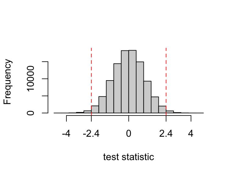
We can see a symmetrical distribution around 0, with most smaller in absolute value than 2.4
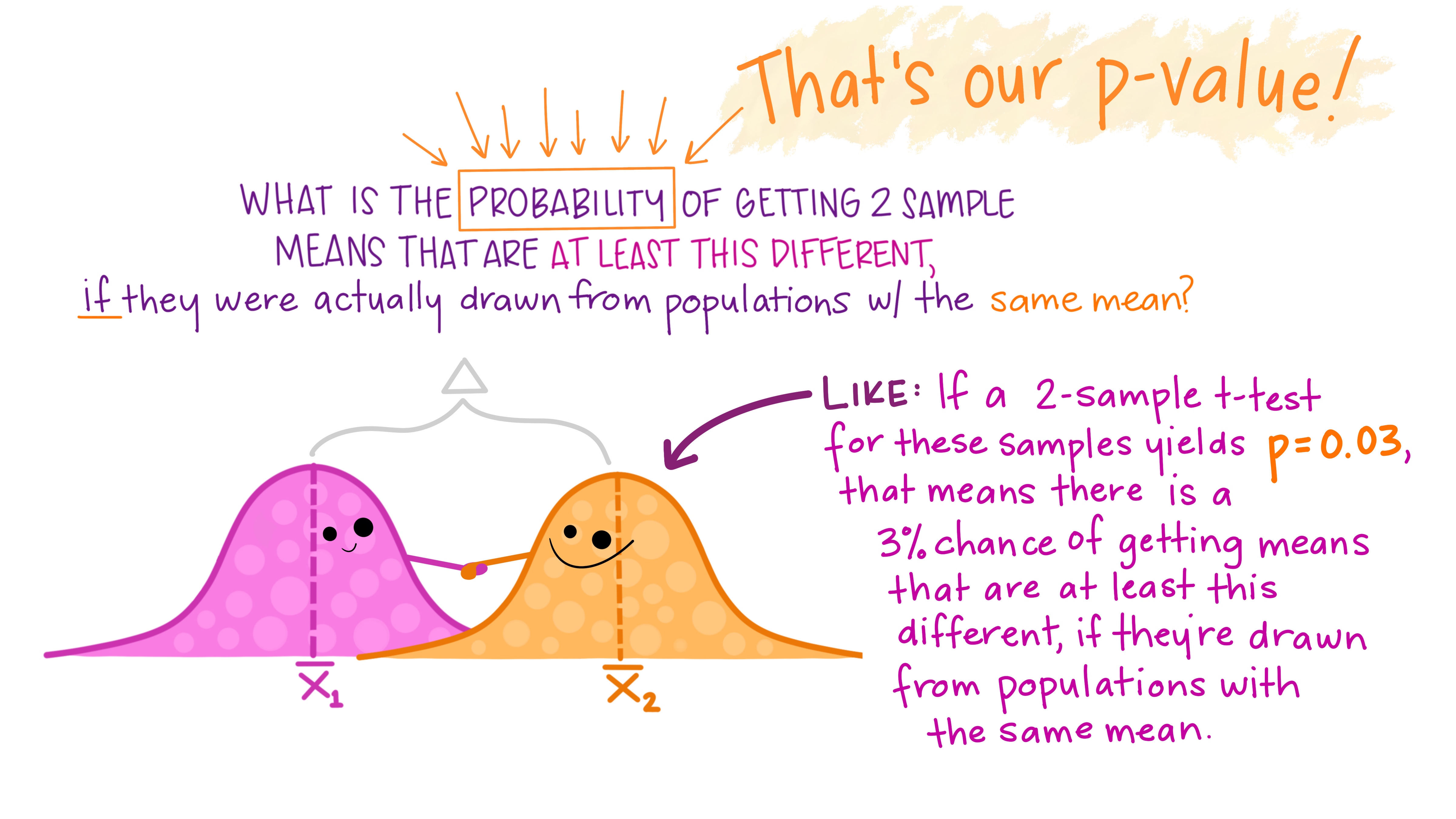
In effect, we’ve computed a \(p\)-value: we’ve used simulation to estimate the probability, assuming \(H_0\) to be true, of getting a test statistic as large as the one we observed.
7.3 The two-sample \(t\) test
As an alternative to the computer simulation, we can use an analytical approach, known as the two-sample \(t\)-test.
Before the experiment has been conducted define \(X_i\) to be the amount that the \(i\)-th participant in the control group will eat, and \(Y_i\) to be the amount \(i\)-th participant in the treatment group will eat. Before the experiment has been conducted, we can think of \(X_i\) and \(Y_i\) as random variables: their values are not yet known.
- The model and hypotheses
We now suppose that
\[\begin{align*} X_1,\ldots,X_{n} &\stackrel{i.i.d}{\sim}N(\mu_X, \sigma^2_X),\\ Y_1,\ldots,Y_{m} &\stackrel{i.i.d}{\sim}N(\mu_Y, \sigma^2_Y), \end{align*}\] so that the population mean amounts eaten under the treatment and control conditions would be \(\mu_X\) and \(\mu_Y\). We consider the hypotheses \[\begin{align*} H_0:\mu_X = \mu_Y,\\ H_A:\mu_X \neq \mu_Y, \end{align*}\] so the null hypothesis is that there is no difference between the mean amount eaten under either condition (it doesn’t matter what the participants imagine doing before they eat.)
- The test statistic, and its distribution under \(H_0\)
We use the test statistic
\[\begin{equation} T = \frac{\bar{X} - \bar{Y} }{\sqrt{\frac{S^2_X}{n} + \frac{S^2_Y}{m} }} \end{equation}\]
Assuming \(H_0\) is true, then approximately \[ T \sim t_\nu, \] i.e \(T\) has a student \(t\) distribution with \(\nu\) degrees of freedom.
As long as the sample sizes are moderately large (say at least 30 per group), this approximation is usually safe to use, even if the individual observations are not normally distributed (the Central Limit Theorem comes into play here).
We will determine \(\nu\) from the data: we use what is known as the Welch approximation \[\begin{equation} \nu = \frac {\left(\frac{s^2_X}{n} + \frac{s^2_Y}{m}\right)^2} {\frac{(s_X^2/n)^2}{n-1} + \frac{(s_Y^2/m)^2}{m-1}}.\tag{7.1} \end{equation}\]
- Computing the \(p\)-value
We compute the value of the test statistic for the observed data
\[t_{obs} = \frac{\bar{x} - \bar{y}}{\sqrt{\frac{s^2_x}{49} + \frac{s^2_y}{47}}} = 2.389.\] and, using the Welch approximation (7.1), we compute the degrees of freedom to be \[ \nu = \frac {\left(\frac{s^2_X}{49} + \frac{s^2_Y}{47}\right)^2} {\frac{(s_X^2/49)^2}{49-1} + \frac{(s_Y^2/47)^2}{47-1}} \simeq 93. \]
To calculate the \(p\)-value, we calculate \[\begin{align*} & P(|T| \ge |t_{obs} |\, | \mbox{$H_0$ true})\\ &= P(|T| \ge 2.4 | \mbox{$H_0$ true})\\ & = P(T \le -2.4 | \mbox{$H_0$ true})\\ &+ P(T \ge 2.4 | \mbox{$H_0$ true}), \end{align*}\] where \(T\) has the \(t_{93}\) distribution under \(H_0\). The \(p\)-value is shown as the red shaded area below. We also show the histogram of test statistics obtained using the simulation method.
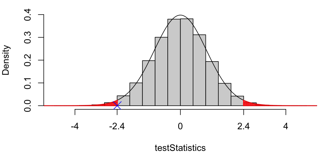
Figure 7.2: The observed test statistic (shown as the blue cross) was -2.4. For the \(p\)-value, we want the probability that \(T\) would be as extreme as this: either less than -2.4, or greater than 2.4. This probability is shown as the red shaded area. For comparison, we also show the histogram of test statistics from the simulation method. Note the close agreement with the \(t\)-distribution.
To calculate the \(p\)-value using R: we want \[\begin{align} &P(T\le - 2.4) + P(T\ge 2.4)\\ &= 2\times P(T\le -2.4) \end{align}\] so the R command to get the \(p\)-value is
2 * pt(-2.4, 93)## [1] 0.01839hence the \(p\)-value approximately 0.02.
To interpret this, we can say that the experiment has provide some evidence that imagining eating food can reduce how much you want to eat! The evidence is not very strong, but this experiment was a replication of an earlier study: two independent studies found the same effect, so taken together, the evidence is more convincing.
7.3.1 The two-sample \(t\)-test with the Neyman-Pearson method
If using the Neyman-Pearson method, we would instead (after choosing the size of the test) identify the critical region. For a test of size 0.05, and a two-sided alternative hypothesis, we would need the 2.5th and 97.5th percentiles of the \(t_\nu\) distribution. Continuing the example, in R, we would do
qt(0.975, 93)## [1] 1.986so the critical region would be \((-\infty, -1.99]\cup [1.99, \infty)\), as shown below.
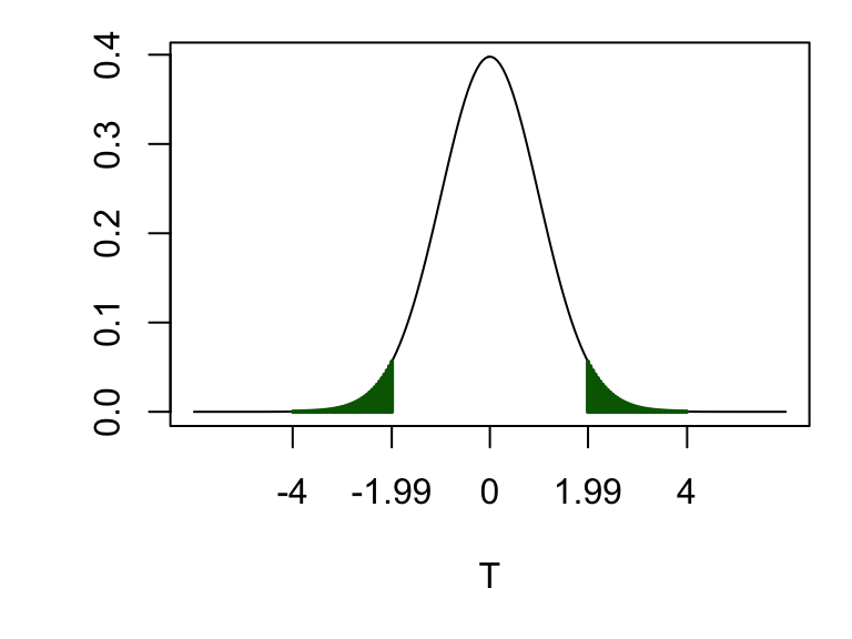
Figure 7.3: The critical region for a test of size 0.05 is shown as by the green shaded area. (The observed test statistic was 2.4, which does fall in this region, so if using the Neyman-Pearson framework, we would conclude that \(H_0\) is rejected at the 5% level of significance.

7.4 Confidence interval for the difference between two means
In addition to reporting the \(p\)-value, we should also report a confidence interval for \(\mu_X - \mu_Y\): what was the difference in means between the two groups?
Sometimes, two groups may be statistically significantly different, but the actual difference may be so small as to be unimportant. Report a confidence interval as well as a \(p\)-value.
The formula for the confidence interval is \[ \bar{x} - \bar{y} \pm t_{\nu,\, 0.025}\sqrt{\frac{s^2_X}{n} + \frac{s^2_Y}{m}}. \] where the degrees of freedom \(\nu\) is the same as that used in the hypothesis test. Substituting in the values, we find this confidence interval to be \([0.74, 7.8]\)g. One M&M weighs about 1g, so the difference in population mean consumption might be somewhere between 1 and 8 M&Ms (at the lower limit, the effect of imagining eating M&Ms could be very small.)
7.5 Equivalence of confidence intervals and Neyman-Pearson testing
A \(100(1-\alpha)\%\) confidence interval for \(\mu_X = \mu_Y\) contains 0 if and only if the null hypothesis \(H_0:\mu_X = \mu_Y\) (with a two-sided alternative) is not rejected in a Neyman Pearson test of size \(\alpha\).
If we have already calculated a \(100(1-\alpha)\%\) confidence interval for \(\mu_X - \mu_Y\), there is no need to do a separate calculation to perform a Neyman Pearson test (of size \(\alpha\)) of the hypothesis \(H_0:\mu_X = \mu_Y\): we simply look to see whether the confidence interval contains the value \(0\) or not.
See the tutorial exercises for a proof.
7.6 The two-sample \(t\) test in R
In R, we use the command t.test(). The two samples we want to compare are stored in the vectors treatment and control, so we do
t.test(control, treatment)##
## Welch Two Sample t-test
##
## data: control and treatment
## t = 2.4, df = 93, p-value = 0.02
## alternative hypothesis: true difference in means is not equal to 0
## 95 percent confidence interval:
## 0.7364 7.8263
## sample estimates:
## mean of x mean of y
## 12.388 8.106We can see in the output the value of the observed test statistic t, the degrees of freedom in the Welch approximation df, the \(p\)-value, as well as a 95% confidence interval for \(\mu_X - \mu_Y\).
7.6.1 \(t\)-tests with data frames in R
If your data are in a data frame, you can use a different syntax which is more convenient. Suppose the data are stored in a data frame called eating, with the first three and last three rows shown below
head(eating, n = 3)## # A tibble: 3 × 2
## group amount
## <chr> <dbl>
## 1 Control 2
## 2 Control 8
## 3 Control 11tail(eating, n = 3)## # A tibble: 3 × 2
## group amount
## <chr> <dbl>
## 1 Treatment 5
## 2 Treatment 6
## 3 Treatment 12The column group indicated which group each participant was in. We can then use the command
t.test(amount ~ group, data = eating)##
## Welch Two Sample t-test
##
## data: amount by group
## t = 2.4, df = 93, p-value = 0.02
## alternative hypothesis: true difference in means between group Control and group Treatment is not equal to 0
## 95 percent confidence interval:
## 0.7364 7.8263
## sample estimates:
## mean in group Control mean in group Treatment
## 12.388 8.106which we can see has produced the same result. (Read the command t.test(amount ~ group, data = eating) as, “do a two-sample \(t\)-test to see if the mean value of the amount variable is different between the groups labelled by the group column, using the data frame eating”).
7.7 Examples
7.7.1 Using the \(p\)-value method
Can social media be bad for your mental health and well-being? This is not a question we would expect to answer definitely with a single experiment; we would not attempt to “reject” or “not reject” a suitable hypothesis once-and-for-all. Rather, we might use hypothesis testing with the \(p\)-value method to help understand the strength of evidence provided by any single experiment.
Example 7.1 (Hypothesis testing: two-sample $t$ test ($p$-value method). Is quitting Facebook good for you?)
Tromholt (2016)8 investigated whether quitting Facebook can improve your well-being.
In the experiment, about a thousand volunteers (all Facebook users) were randomly allocated to either a treatment group, in which they told not to use Facebook for one week, or a control group, in which they carried on using Facebook as normal. At the end of the week, all participants completed a questionnaire. One of the questions asked them to record, “In general, how satisfied are you with your life today?” on a scale of 1 (very dissatisfied) to 10 (very satisfied). Let \(x_1,\ldots,x_n\) be the observed responses in the treatment group, and \(y_1,\ldots,y_m\) be the observed responses in the control group. Results from those who repsponded were as follows.
\[ \bar{x} = 8.11,\, \bar{y} = 7.74,\, s^2_X = 1.23^2,\, s^2_Y = 1.43^2,\,n = 516, \,m=372 \] with
\[ \nu = \frac {\left(\frac{s^2_X}{516} + \frac{s^2_Y}{372}\right)^2} {\frac{(s_X^2/516)^2}{516-1} + \frac{(s_Y^2/372)^2}{372-1}} \simeq 726. \]
- Defining your notation carefully, state suitable hypotheses for the experiment.
- Conduct an appropriate hypothesis test, reporting the \(p\)-value.
- Report a 95% confidence interval for the difference in population means.
- In plain English, summarise your results.
Some R output to help is as follows:
pt(-4.03, 726)## [1] 3.083e-05qt(0.975, 726)## [1] 1.963Solution
- Define \(\mu_X\) to be the population mean “life satisfaction score” under the treatment group condition, and \(\mu_Y\) to be the population mean score under the control group condition. Our hypotheses are
\[\begin{align*} H_0: \mu_X &= \mu_Y,\\ H_A: \mu_X &\neq \mu_Y. \end{align*}\]
- Using the two-sample \(t\)-test, we compute \[t_{obs} = \frac{\bar{x} - \bar{y}}{\sqrt{\frac{s^2_x}{516} + \frac{s^2_y}{372}}} = 4.03.\] For the degrees of freedom parameter, we are given \(\nu\simeq726\), so under \(H_0\), the test statistic would have (approximately) a \(t_{726}\) distribution.. The observed test statistic is right out in the tail of this distribution, so the \(p\)-value will be small.
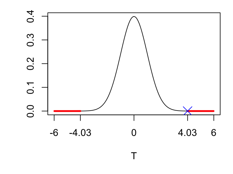
The \(p\)-value is given by \[ 2 \times P(T_{726} \le -4.03) \simeq 6\times 10^{-5} \]
An approximate 95% confidence interval for the difference in population means is \[ \bar{x} - \bar{y} \pm t_{726,\, 0.025}\sqrt{\frac{s^2_X}{n} + \frac{s^2_Y}{m}}. \] From the R output, we have \(t_{726,\, 0.025}=1.963\), so the confidence interval is \([0.2, 0.6]\), to 1 decimal place.
The experiment found very strong evidence against the null hypothesis of equal mean life satisfaction scores, with the particants who did not use Facebook for one week giving higher scores. However, the effect of not using Facebook was small: the difference in means is likely less than a single point on the 10 point response scale.
7.7.2 Using Neyman-Pearson testing
Neyman-Pearson testing is used is in medical research, specifically, clinical trials for new drugs. The scenario would be something like this:
- A pharmaceutical company has developed a new drug, and will test it using a hypothesis test.
- The null hypothesis is that the drug has no effect.
- The action to be taken following the test is either to license the drug for use on patients, or to decide that it cannot be used; the pharmaceutical company would then abandon that drug, and move onto to developing a different drug.
- If the null hypothesis is “rejected”, we conclude that the drug does has an effect, and the drug gets its license (assuming the drug effect is beneficial for patients).
- If the null hypothesis is “not rejected”, we conclude that there is no evidence the drug works, and it is not licensed for further use.
Example 7.2 (Hypothesis testing: two-sample $t$ test (Neyman-Pearson method). Testing a new diabetes treatment.)
Patients with type-2 diabetes may use drugs to control their blood sugar levels. A pharmaceutical company (Merck) conducted a clinical trial to compare the efficacy of a combination of two drugs, sitagliptin and metformin, with using metformin alone. The product name for this combination of drugs is “Efficib”. 190 patients were recruited to the trial, and were randomly allocated to one of two treatments:
- treatment 1: 100mg sitagliptin per day, and at least 1500mg metformin per day
- treatment 2: a daily placebo, made to look like a dose of 100mg sitagliptin, and at least 1500mg metformin per day.
The study was “double-blinded”: neither the patients nor their doctors knew which treatment they were getting (though the trial investigators did know.) A1C (a measure of blood sugar level) was recorded for each patient at the start and after 18 weeks, and the change in A1C was recorded for each patient.
We model this as follows.
Let \(X_i\) denote the change in A1C for the \(i\)-th patient on the treatment 1, and \(Y_i\) denote the change in A1C the \(i\)-th patient on treatment 2. We suppose \[\begin{align*} X_1,\ldots,X_{95}&\stackrel{i.i.d}{\sim}N(\mu_X, \sigma^2_X),\\ Y_1,\ldots,Y_{92}&\stackrel{i.i.d}{\sim}N(\mu_Y, \sigma^2_Y). \end{align*}\]
We denote the corresponding observed values by \(x_1,\ldots,x_{95}\) and \(y_1, \ldots, y_{92}\). The trial results are published at clinicaltrials.gov. Individual patient data are not normally published, and we can infer (approximately) what the summary statistics were: we have
\[\begin{align} \bar{x} &= \frac{1}{95}\sum_{i=1}^{95}x_i = -1.00,\\ s^2_X &= \frac{1}{94}\sum_{i=1}^{95}(x_i - \bar{x})^2= 1.5456,\\ \bar{y} &= \frac{1}{92}\sum_{i=1}^{92}y_i = 0.02,\\ s^2_Y &= \frac{1}{91}\sum_{i=1}^{92}(y_i - \bar{y})^2= 1.4968. \end{align}\]
- State appropriate null and hypotheses, in terms of your model parameters, to test whether the addition of sitagliptin had an effect
- Conduct an appropriate Neyman-Pearson test, of size 0.05, stating the conclusions clearly.
Some R output to help is as follows.
qt(c(0.9, 0.95, 0.975, 0.99), 185)## [1] 1.286 1.653 1.973 2.347Solution
We consider the hypotheses \[\begin{align*} H_0 &: \mu_X = \mu_Y,\\ H_A &: \mu_X \neq \mu_Y, \end{align*}\] so that the null hypothesis is that there is no effect from the additional treatment with sitagliptin
For our two-sample \(t\)-test, we have \[ t_{obs}=\frac{\bar{x} - \bar{y}}{\sqrt{\frac{s^2_X}{95} + \frac{s^2_Y}{92}}} = -5.655, \]
\[ \nu = \frac {\left(\frac{s^2_X}{95} + \frac{s^2_Y}{92}\right)^2} {\frac{(s_X^2/95)^2}{94} + \frac{(s_Y^2/92)^2}{91}} \simeq 185. \] Hence, for a test of size 0.05, our critical region is anything above \(t_{185;\, 0.025}\) or anything below \(t_{185;\, 0.975}\) (anything above the 97.5th percentile, or anything below the 2.5th percentile, for the student-\(t\) distribution with 185 degrees of freedom.) From the R output, we have \(t_{17.7;\, 0.025}=1.97\) and so \(t_{17.7;\, 0.975}=-1.97\). The critical region and observed test statistic are plotted below.
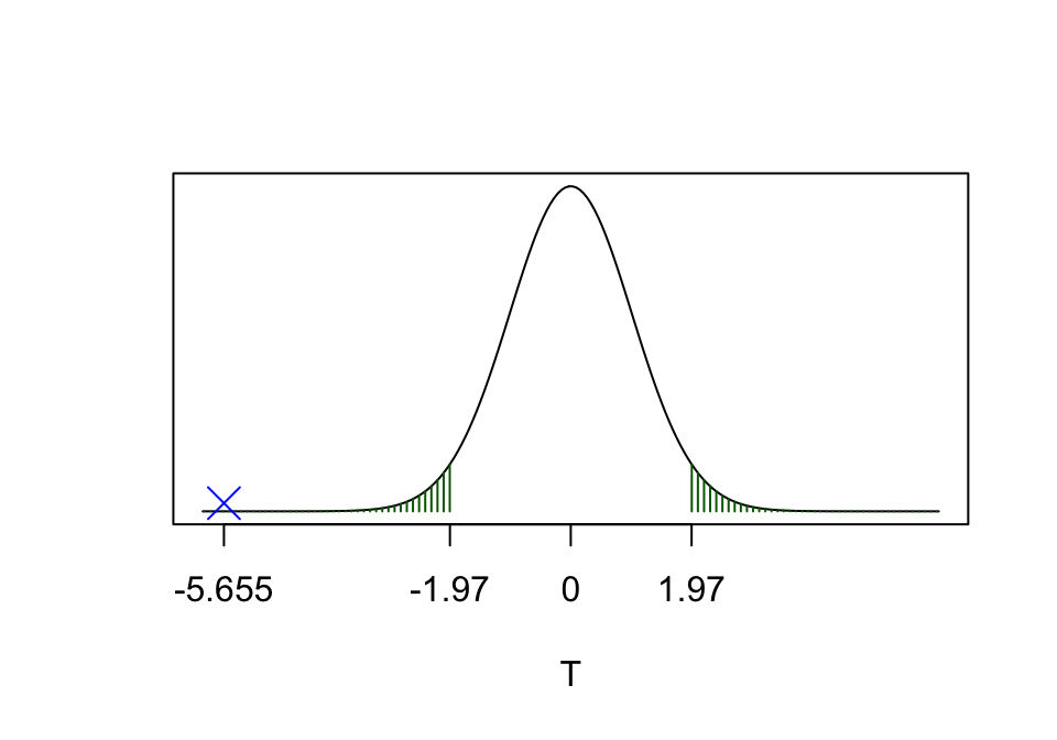
Figure 7.4: \(t_{obs}\) for the observed data is calculated to be -5.655, and is shown as the blue cross. This does lie in the critical region (the green shaded area), so we declare that ‘we reject \(H_0\) (at the 5% level of significance)’.
As \(t_{obs}\) does lie in the critical region, we conclude that we reject \(H_0\). We say that there is evidence (at the 5% level of significance) that there is an effect of combining sitagliptin with metformin, and that this effect is an increased reduction in A1c (adding sitagliptin has a beneficial effect.)
There have been other studies to test the effect of sitagliptin and metformin (the “Efficib” drug). Based on these studies, the European Medicines Agency approved Efficib for use in the European Union.
Morewedge, C. K., Huh, Y. E. & Vosgerau, J. Thought for food: imagined consumption reduces actual consumption. Science 330, 1530–1533 (2010).↩︎
Camerer, C. F., Dreber, A., Holzmeister, F., Ho, T.-H., Huber, J., Johannesson, M.,… Wu, H. (2018). Evaluating the replicability of social science experiments in Nature and Science between 2010 and 2015. Nature Human Behaviour, 2(9), 637–644. https://doi.org/10.1038/s41562-018-0399-z↩︎
Morten Tromholt Cyberpsychology, Behavior, and Social Networking 2016 19:11, 661-666.↩︎