Chapter 2 Machine Learning

The term “Machine Learning” was used in a paper by Arthur Samuel in 1959¹, on how a computer could learn to play a better game of checkers. In general machine learning involves getting a computer to ‘learn from experience’, so that it can perform a particular task in a new situation without being programmed what to do. Machine learning underpins technology described as “artificial intelligence”.

Some machine learning problems involve getting computers to recognise speech, read handwriting, and identify objects in images. More recently, machine learning methods have been used to analyse very large and complex data sets, where the scale of the problem is too large for humans to manage (e.g. recommending products to millions of individual customers, based on vast databases of customer purchases).

This chapter will give a short introduction, where we will look at a single problem and method, and we will consider the role of data analysis within machine learning.

2.1 Can we teach a computer to identify handwritten digits?

Below are some scanned images of handwritten digits. The images are from the (well-known) “MNIST” data set, hosted on Yann Lecun’s website.

We can see what the digits are without too much difficulty, but can we get a computer to recognise the digits?

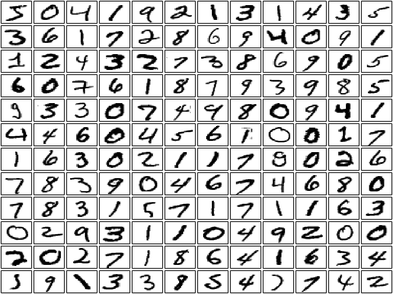
Figure 2.1: Scanned images of hand-written digits (not all written by the same person). We can easily recognise what the digits are: could a computer do so?

The key idea is to make this a data analysis problem. The steps are as follows.

1. Convert the objects we want the computer to recognise (the scanned images) into numerical data: find a way to represent each image with a set of numbers. The computer will need to be able to do this conversion automatically, without knowing what each digit in a scanned image actually is.
2. Construct a training data set: a (large) data set of example handwritten digits, all converted into numerical data. In addition, we also tell the computer what each handwritten digit is: “The first image in the data set is the number 5, the second image in the number 0,” and so on.
3. Construct a statistical model or algorithm using the training data set, that given an image in its converted numerical form, can estimate what the handwritten digit is.

In this module, steps 1 and 2 will always be done for you; you will only need one method for doing step 3.

2.1.1 Step 1: converting an image into data

(The images first need to be scaled to the same size, with the handwriting approximately in the centre of the image. This step has been done for us.)

Here is one example image:

Figure 2.2: A single scanned image of a handwritten digit. (The top left corner image from Figure 2.1.) Zooming in, we can see that the image is made up of shaded blocks.

The image is made up of pixels (shaded dots), arranged on a 28x28 grid (these are low resolution images!) The shading of each pixel can be represented numerically, on a scale of 0 (white) to 255 (black).

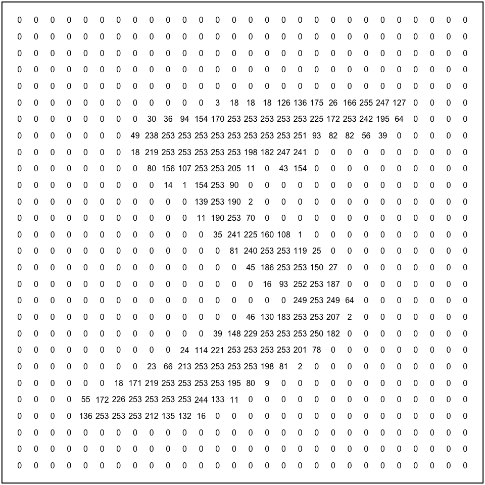
Figure 2.3: This is how the computer ‘sees’ the image, as a grid of pixel shades (here with higher numbers representing darker shades). We can use these numbers to represent the image in numerical form.

We can now represent the image by a vector \(\mathbf x\) with \(28^2 = 784\) elements: \[\mathbf x = (x_1,x_2,\ldots,x_{784}),\] taking one row at a time from the above image. Starting with the top row, the vector would look like this: \[ \mathbf x=(0,0,0,\ldots,0,0, 0,3, 18, 18, 18, 126, 136,\ldots, 135, 132, 16, 0, 0, \ldots, 0, 0, 0) \]

2.1.2 Step 2: assembling the training data set

We now assemble a training data set of 60,000 images. The \(i\)-th image in the data set is represented by the vector \(\mathbf x_i\), where \[ \mathbf x_i = (x_{i,1},x_{i,2},\ldots,x_{i,784}) \] We define \(y_i\) to be the class label for the \(i\)-th image. In this case, the class label will be a number from 0-9, that says what the hand written digit is. For the training data set, the class labels are simply given to us: we don’t need to work out what they should be. We write the training data set in the form \[(\mathbf x_1,y_1), (\mathbf x_2,y_2),\ldots, (\mathbf x_{60,000}, y_{60,000}).\]

If \((\mathbf x_1, y_1)\) corresponds to the first image in the training data set, then \(\mathbf x_1\) is the vector with elements given by the numbers in Figure 2.3, and \(y_1=5\): the image is a hand-written number 5.

2.1.2.1 Setting up the data in R.

If you want to get the data for yourself, I suggest you download the data in csv format: csv files mnist_train.csv and mnist_test.csv can be downloaded from this site maintained by Joseph Redmon. Once you have downloaded them, assuming the files are in your working directory, use the commands

library(tidyverse)
training_set <- read_csv("mnist_train.csv", col_names = FALSE)
test_set <- read_csv("mnist_test.csv", col_names = FALSE)

For the training data, the class labels \(y_1,y_2,\ldots,y_{60000}\) are stored in the first column of training_set. The image vector \(x_i\) is stored in row \(i\), columns 2 to 725. As well as the training data, we have another data set know as the “test data”, which are stored are stored similarly in test_set.

2.1.3 Step 3: an algorithm for estimating the digit in a new image

We have a separate test data set made up of 10,000 images. We will represent these by the vectors \[ \tilde{\mathbf x}_1,\tilde{\mathbf x}_2,\ldots,\tilde{\mathbf x}_{10,000} \] The first image in our test data set and its numerical representation \(\tilde{\mathbf x}_1\) are shown below.

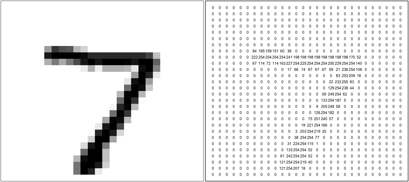
Figure 2.4: The first image in the test data set, represented by a vector \(\tilde{\mathbf x}_1\), with elements made up of the numbers on the right hand side. How can a computer use the training data to tell that this is a number ‘7’?

How to get the computer to recognise that this is a number 7? There are lots of algorithms we could try (and, in general, many statistical models can be used for machine learning). Here, we will use a simple one, known as “\(K\) nearest neighbours”.

2.1.4 The \(K\) nearest neighbour algorithm (KNN)

In the \(K\) nearest neighbours method, the computer will decide what number an image is by looking for similar images in the training data. It can then use the known class labels in the training images to estimate what the new test image is. Writing out the vector

\[ \tilde{\mathbf x}_1 = (\tilde{x}_{1,1},\tilde{x}_{1,2},\ldots,\tilde{x}_{1,784}) \]

we will measure similarity using the (square of) the Euclidean distance between \(\tilde{\mathbf x}_1\) and each training image \(\mathbf x_i\). We define \[ d(\tilde{\mathbf x}_1, \mathbf x_i) := \sum_{j=1}^{784}(\tilde{x}_{1, j} - x_{i,j})^2, \] so the smaller the distance, the more similar the images are. The computer will decide what digit \(\tilde{\mathbf x}_1\) is as follows:

1. Compute \(d(\tilde{\mathbf x}_1, \mathbf x_i)\) for \(i=1,2,\ldots,60000\)
2. Find the nearest neighbour: look for smallest distance out of \[d(\tilde{\mathbf x}_1, \mathbf x_1),\quad d(\tilde{\mathbf x}_1, \mathbf x_2),\, \ldots\,,\,d(\tilde{\mathbf x}_1, \mathbf x_{60000})\]
3. If the nearest neighbour was image \(j\) (the smallest distance was \(d(\tilde{\mathbf x}_1, \mathbf x_j))\), then estimate the digit to be \(y_j\): the known class label for image \(j\).

As an example, we compute

\[\begin{align} d(\tilde{\mathbf x}_1, \mathbf x_1) &= \sum_{j=1}^{784}(\tilde{x}_{1, j} - x_{1,j})^2\\ &= 5,739,837 \end{align}\] We view this below.

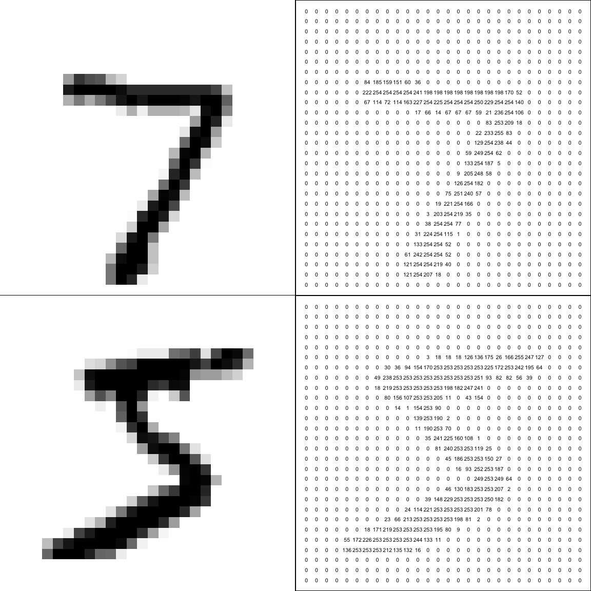
Figure 2.5: Top row: the first test image and its numerical representation \(\tilde{\mathbf x}_1\). Bottom row: the first image in the training data set and its numerical representation \(\mathbf x_1\). To compute the similarity between the images, we square the differences between the numbers at the same corresponding positions in the right hand column, and sum.

We compute \(d(\tilde{\mathbf x}_1, \mathbf x_i)\) for all 60000 images. The image most similar to \(\tilde{\mathbf x}_1\) turns out to be image number 53844 in the training data set: \[\begin{align} d(\tilde{\mathbf x}, \mathbf x_{53844}) &= \sum_{j=1}^{784}(\tilde{x}_{1, j} - x_{53844,j})^2 \\ &=457,766 \end{align}\] We view this below.

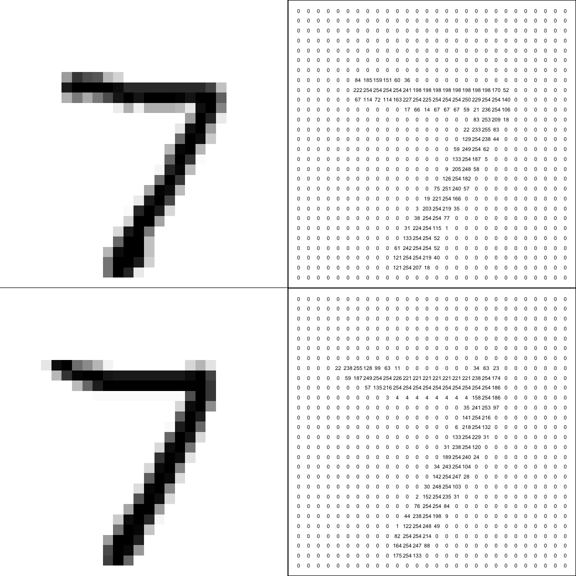
Figure 2.6: Top row: the first test image and its numerical representation \(\tilde{\mathbf x}_1\). Bottom row: image number 53844 in the training data set and its numerical representation \(\mathbf x_{53844}\). To compute the similarity between the images, we square the differences between the numbers at the same corresponding positions in the right hand column, and sum. By this measure of similarity, image 53844 is closest to our test image.

So, the computer will look up the value of \(y_{53844}\) in the training data set, which is recorded as 7, and so estimate the test image to be the number 7.

2.1.4.1 The ‘\(K\)’ in \(K\) nearest neighbours

We’ve actually used the simplest version of the KNN algorithm, where we look for the single nearest neighbour. An extension is to look for the \(K\) nearest neighbours, and then choose the class label based on which which label occurs the most out of the \(K\) nearest neighbours (so we have just used \(K=1\) above). This may give better results, for example, if there is the odd ‘badly drawn’ image in the training data set, that looks like a different digit: it can be out-voted if we search for more nearest neighbours.

2.1.5 Using \(K\) nearest neighbours in R

We can use the function knn() from the package class.

2.1.5.1 A simple example

We’ll first do a simple example on a small data set, to make it easier to see how everything works.

(Ignore the following three commands, unless you want to try this on your own computer. These commands will make the data we are going to use for the example.)

irisTrain <- iris[c(1, 6, 51, 52, 101, 102), 3:5]
irisTest <- cbind(flower = c("A", "B"),
                  iris[c(44, 53), 3:4]) 
row.names(irisTrain) <- row.names(irisTest) <- NULL

In our training data, a data frame called irisTrain, we have observations of the lengths and widths of petals for 6 flowers (species of iris). Each flower is one of three possible species: setosa, versicolor, or virginica.

irisTrain

##   Petal.Length Petal.Width    Species
## 1          1.4         0.2     setosa
## 2          1.7         0.4     setosa
## 3          4.7         1.4 versicolor
## 4          4.5         1.5 versicolor
## 5          6.0         2.5  virginica
## 6          5.1         1.9  virginica

In our test data, irisTest, we have two iris flowers, labelled A and B, with measured petal lengths and widths: the aim is to predict the species of these two flowers.

irisTest

##   flower Petal.Length Petal.Width
## 1      A          1.6         0.6
## 2      B          4.9         1.5

If we plot the training and test data together, we can see that the closest flower in the training data to flower A has species setosa, and the closet flower in the training data to flower A has species versicolor, so we would predict that flowers A and B are species setosa and versicolor respectively.

ggplot(irisTrain, aes(x = Petal.Length,
                      y = Petal.Width))+
  geom_point(aes(color = Species)) +
  annotate("text", x = irisTest$Petal.Length,
           y = irisTest$Petal.Width,
           label = irisTest$flower)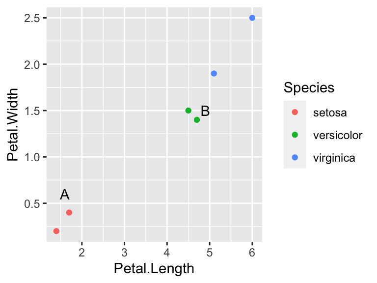

Figure 2.7: The training data are shown as the 6 coloured points. The test data are marked as the two letters. The nearest neighbour to flower A has species setosa, and the nearest neighbour to flower B has species versicolor.

To use the KNN algorithm in R, we use the function knn() from the class library. We specify three arguments:

• train: the measurements in the training data, excluding the class labels (the Species column). We need to exclude column 3, which we can do as follows:

irisTrain[, -3]

##   Petal.Length Petal.Width
## 1          1.4         0.2
## 2          1.7         0.4
## 3          4.7         1.4
## 4          4.5         1.5
## 5          6.0         2.5
## 6          5.1         1.9

• test: the measurements in the test data. We will need to exclude the flower labels. These labels are also in the first column, so we do

irisTest[, -1]

##   Petal.Length Petal.Width
## 1          1.6         0.6
## 2          4.9         1.5

• cl: the class labels in the training data. These are in the Species column, so we can extract these using

irisTrain$Species

## [1] setosa     setosa     versicolor versicolor virginica  virginica 
## Levels: setosa versicolor virginica

So, we use the knn() function as follows:

library(class)
knn(train = irisTrain[, -3], 
    test = irisTest[, -1],
    cl = irisTrain$Species)

## [1] setosa     versicolor
## Levels: setosa versicolor virginica

So, out of the three possible Levels, the KNN algorithm classifies flower A as setosa and flower B as versicolor. This agrees with what we could see in Figure 2.7

2.1.5.2 Using knn() with the handwritten digits

Returning to the handwritten digits, suppose we have the training images and class labels stored in a single data frame called training_set, where each row is one image, with the class label in column 1 and the pixel values in columns 2 to 785. We display the first 5 columns below:

training_set[, 1:5]

## # A tibble: 60,000 × 5
##       X1    X2    X3    X4    X5
##    <dbl> <dbl> <dbl> <dbl> <dbl>
##  1     5     0     0     0     0
##  2     0     0     0     0     0
##  3     4     0     0     0     0
##  4     1     0     0     0     0
##  5     9     0     0     0     0
##  6     2     0     0     0     0
##  7     1     0     0     0     0
##  8     3     0     0     0     0
##  9     1     0     0     0     0
## 10     4     0     0     0     0
## # … with 59,990 more rows

(Look at the first column, and compare it with the first row in Figure 2.1, which shows the first 10 images in the training data set.)

We now extract the class labels and images as follows:

training_images <- training_set %>%
  select(-X1)

The minus sign means that we select all columns apart from X1. We then extract the class labels:

training_labels <- training_set$X1

Suppose the test set are arranged in another data frame test_set, with the same structure. We then extract the images:

test_images <- test_set %>%
  select(-X1)

Now we can use the knn() function. We’ll just use it on the first 5 images in the test set:

library(class)
knn(train = training_images,
    test = test_images[1:5, ],
    cl = training_labels)

## [1] 7 2 1 0 4
## Levels: 0 1 2 3 4 5 6 7 8 9

(The first row of the output means that the algorithm estimates the first five digits to be 7, 2, 1, 0, 4. The second row gives the full range of digits provided in training_labels.) Inspecting the first five test images, we can see that the algorithm has worked!

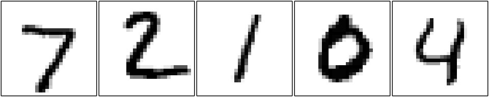
Figure 2.8: The first five images in the test set. We can see that algorithm has correctly identified all five digits.

2.1.6 The performance of the algorithm

The algorithm won’t always get it right! Here’s an example where the algorithm gets it wrong (test image number 116):

knn(train = training_images,
    test = test_images[116, ],
    cl = training_labels)

## [1] 9
## Levels: 0 1 2 3 4 5 6 7 8 9

After a little investigation (details omitted), it turns out that image 8112 in the training data is closest to image 116 in the test data. If we look at the image, we can see where the algorithm went wrong: the test image is a ‘4’, but it looks very similar to a ‘9’ in the training data.

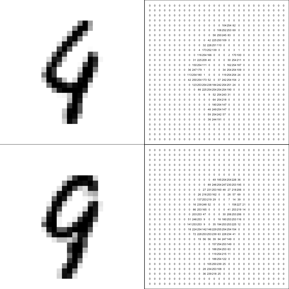
Figure 2.9: Top row: test image 116 and its numerical representation \(\tilde{\mathbf x}_{116}\). Bottom row: image number 8112 in the training data set and its numerical representation \(\mathbf x_{8112}\). This training image is the closest to our test image, but the digits are not the same!

Applying the algorithm to all 10000 test images, the algorithm gets the right answer 9691 times (96.91%). This may look quite good, but an error rate of 3% is probably too large in practice. But the performance is good enough to show the potential of using a data-based method for the image recognition problem. In fact, more complex methods do give better performance. A list of results is maintained here, with the best performing method (at the time of writing) being 99.79% accurate.

---

1. Samuel, Arthur (1959). Some Studies in Machine Learning Using the Game of Checkers. IBM Journal of Research and Development. 3 (3): 210-229.↩︎