Chapter 4 Point estimation
In this chapter, we consider how to estimate the parameters of a probability distribution, given observations from that distribution. By “point” estimate, we mean a single number as the estimate. (In the next chapter, we will consider interval estimates: estimates in the form of a range of values).
4.1 Estimating the parameters of a normal distribution
4.1.1 Problem setup and notation
Suppose we model some data with a normal distribution: we have \(n\) independent and identically distributed normal random variables \[\begin{equation} X_1,X_2,\ldots,X_{n}\stackrel{i.i.d}{\sim} N(\mu, \sigma^2), \end{equation}\] where the values of \(\mu\) and \(\sigma^2\) are unknown to us. We denote the observed values of these \(n\) random variables by \(x_1,\ldots,x_n\). How should we estimate \(\mu\) and \(\sigma^2\) using \(x_1,\ldots,x_n\)? This problem is illustrated in Figure 4.1.
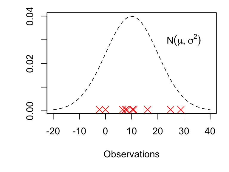
Figure 4.1: The red crosses show 10 observations drawn from the \(N(\mu, \sigma^2)\) distribution. Suppose we only know the values of these 10 observations: can we use them to estimate the values of \(\mu\) and \(\sigma^2\)?
The distinction between big \(X\) and little \(x\) is important: we use \(X_i\) to represent a random variable, and \(x_i\) to represent the observed value of a random variable.
We can think of \(X_i\) as describing the situation before we have collected our data: we don’t know what value we are going to observe, so we represent it by a random variable \(X_i\).
We can think of \(x_i\) as describing the situation after we have collected our data: we now have a numerical value for our \(i\)th observation, which we denote by a constant \(x_i\).
4.1.2 The sample mean and sample variance
We’ll define some notation/terminology now, that we will use a lot from now on.
Definition 4.1 (Sample mean) Given the observations \(x_1,\ldots,x_n\), we define the sample mean to be \[ \bar{x}: = \frac{1}{n}\sum_{i=1}^n x_i. \]
Definition 4.2 (Sample variance) Given the observations \(x_1,\ldots,x_n\), we define the sample variance to be \[ s^2: = \frac{1}{n-1}\sum_{i=1}^n (x_i-\bar{x})^2. \]
Confusingly, the word “mean” has multiple meanings in probability and statistics! Don’t confuse the “sample mean” \(\bar{x}\) with the “mean of a random variable” \(\mathbb{E}(X)\): they are not the same thing! Similarly, “sample variance” doesn’t mean the same thing as the “variance of a random variable” \(Var(X)\)
4.1.3 Point estimates for the mean and variance
For now, we will simply state suitable estimates for the parameters of any distribution (methods such as “maximum likelihood estimation” can be used to derive estimates). For the normal distribution, we will use the estimates
\[\begin{align} \hat{\mu} &:= \bar{x} \\ \hat{\sigma}^2 &:= s^2. \end{align}\]
The hat \(\hat{}\) notation is important here: it is used to denote that \(\hat{\mu}\) and \(\hat{\sigma}^2\) are only estimates of \(\mu\) and \(\sigma^2\). Don’t write an expression such as \(\mu = \bar{x}\): this would be claiming that the true value of the unknown mean parameter \(\mu\) is the sample mean \(\bar{x}\).
In R, these can be calculated with the functions mean() and var() respectively.
4.1.4 Testing the method
To illustrate the notation, the R commands, and to persuade ourselves that the formulae give sensible estimates, we’ll do a simulation example in R.
We’ll consider a sample of 100 observations
\[ X_1,\ldots, X_{100}\stackrel{i.i.d}{\sim} N(\mu, \sigma^2) \] We’ll now get R to generate some data. To do this, we have to choose values for \(\mu\) and \(\sigma^2\): I’ll choose \(\mu=20\) and \(\sigma^2 = 25\):
x <- rnorm(n = 100, mean = 20, sd = 5)If we inspect the first three elements of x, we get
x[1:3]## [1] 20.36 16.76 16.07so we have \(x_1=\) 20.36, \(x_2=\) 16.76, \(x_3=\) 16.07, \(\ldots\). Now pretending that we don’t know the true values of \(\mu\) and \(\sigma^2\), we compute our sample mean and sample variance:
mean(x)## [1] 18.89395var(x)## [1] 30.37141so we have \[\begin{eqnarray*} \hat{\mu}&=& \bar{x} = \frac{1}{100}\sum_{i=1}^{100} x_i=\mbox{18.9},\\ \hat{\sigma}^2&=& s^2 = \frac{1}{99}\sum_{i=1}^{100} (x_i-\bar{x})^2= \mbox{30.4}, \end{eqnarray*}\] to 3 s.f., and these estimates are similar to the true values, as we would hope. We illustrate this in Figure 4.2.
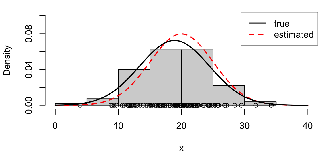
Figure 4.2: The circles and histogram represent 100 observations drawn from the \(N(\mu, \sigma^2)\) distribution. We display the true normal distribution with the red dashed line. We compute estimates of \(\mu\) and \(\sigma^2\) using \(\bar{x}\) and \(s^2\): the corresponding estimated normal distribution is shown as the black curve, and is fairly similar to the true distribution: the estimates are fairly similar to the true values.
4.1.5 Estimators and estimates
Over the next few sections, we will explain why \(\bar{x}\) and \(s^2\) were good choices of estimates to use for \(\mu\) and \(\sigma^2\).
As a motivating example, suppose we are planning an experiment to test a new steel manufacturing process. A batch of \(n\) steel cables will be produced, and the tensile strength of each cable will be measured. We don’t yet know what the tensile strengths will be, and we denote the strength of the \(i\)th cable by the random variable \(X_i\). We suppose that the strengths are normally distributed: \[\begin{equation} X_1,X_2,\ldots,X_{n}\stackrel{i.i.d}{\sim} N(\mu, \sigma^2), \end{equation}\] and the aim of the experiment is to estimate \(\mu\) and \(\sigma^2\).
Although we don’t yet have the data, we are going to declare now how we intend to estimate \(\mu\) and \(\sigma^2\), and then investigate whether our estimation method is likely to ‘work’ or not: whether it is likely to produce good estimates.
We declare that we are going to use the following two estimators, to estimate \(\mu\) and \(\sigma^2\) respectively: \[\begin{align} \bar{X} &:= \frac{1}{N}\sum_{i=1}^n X_i,\\ S^2 &:= \frac{1}{n-1}\sum_{i=1}^n (X_i-\bar{X})^2. \end{align}\]
Definition 4.3 (Estimators) An estimator is a function of some random variables \(X_1,\ldots,X_n\) intended to provide an estimate of some parameter from the distribution of \(X_1,\ldots,X_n\).
Don’t confuse \(\bar{X}\) and \(S^2\) with \(\bar{x}\) and \(s^2\)! Both \(\bar{X}\) and \(S^2\) are random variables because they are functions of the random variables \(X_1,\ldots,X_n\).
An estimator is a random variable; the observed value of the estimator, calculated using the observed values \(x_1,\ldots,x_n\) is the corresponding estimate.
In our steel cables example:
- we haven’t yet done the experiment; the cables haven’t been manufactured yet, and we can’t know what values for the tensile strengths we will observe. At this stage, we think of the \(n\) tensile strengths \(X_1,\ldots,X_n\) as random variables, so both \(\bar{X}\) and \(S^2\) are random too.
- After we have done the experiment, we will have the \(n\) numerical values for the tensile strengths, and the sample mean and variance that we calculate from these values will be represented by the constants \(\bar{x}\) and \(s^2\).
Now we can ask the question: are \(\bar{X}\) and \(S^2\) good estimators? Given that they are random variables, how likely is it that they will give us values ‘close’ to the true values of \(\mu\) and \(\sigma^2\)?
4.1.6 The \(\chi^2\) distribution
We’ll shortly discuss the distribution of the two estimators \(\bar{X}\) and \(S^2\), but first, we need to introduce a new distribution.
Definition 4.4 ($\chi^2$ distribution) If a random variable \(Y\) has the \(\chi^2_\nu\) distribution (the “chi-squared distribution with \(\nu\) degrees of freedom”), we write \(Y\sim \chi_\nu^2\) and the probability density function of \(Y\) is given by \[\begin{equation}\label{chisquare2} f_Y(y) = \left\{\begin{array}{cc}\frac{y^{\nu/2-1}}{2^{\nu/2} \Gamma(\nu/2) } \exp\left(-\frac{y}{2}\right),& y\geq 0,\\ 0 & y<0.\end{array}\right. \end{equation}\] Note that we must have \(\nu>0\). Here \(\Gamma\) denotes the gamma function, defined by \[\begin{equation} \Gamma(x)=\int_0^{\infty}t^{x-1}e^{-t}dt. \end{equation}\]
It can be shown that \[\begin{align} \mathbb{E}(Y)&= \nu,\tag{4.1}\\ Var(Y)&=2\nu.\tag{4.2} \end{align}\] The \(\chi^2_\nu\) distribution is positively skewed, with the skew more apparent as the degrees of freedom \(\nu\) decreases. Three \(\chi^2\) distributions are plotted in Figure 4.3.
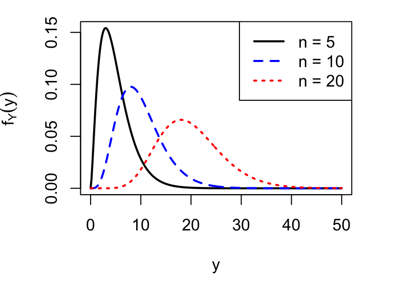
Figure 4.3: Three \(\chi^2_{n}\) distributions with \(n=5\), 10 and 20 degrees of freedom.
We won’t be working with the density function of the \(\chi^2\) distribution in this module, but you will need to know its mean and variance, and that a \(\chi^2\) random variable cannot be negative.
4.1.7 The distribution of the estimators
As the estimators are random variables, we can derive their probability distributions. It can be shown that:
\[\begin{equation} \bar{X}\sim N\left(\mu, \frac{\sigma^2}{n}\right)\tag{4.3} \end{equation}\]
For the distribution of \(S^2\), we have the following result. If define the random variable \(R\) to be \[\begin{equation} R:=\frac{(n-1)S^2}{\sigma^2}, \end{equation}\] then \(R\) has the probability distribution \[\begin{equation} R \sim \chi^2_{n-1}. \tag{4.4} \end{equation}\] You can learn how to prove this result in MAS223. For now, we’ll just note that \(\frac{(n-1)S^2}{\sigma^2}\) cannot be negative, which is one property of the \(\chi^2\) distribution.
4.1.8 Unbiased estimators
We can now justify why \(\bar{X}\) and \(S^2\) are good choices of estimators for \(\mu\) and \(\sigma^2\).Definition 4.5 (Unbiased estimator) Let \(T(X_1,\ldots,X_n)\) be a function of \(X_1,\ldots,X_n\). We say that \(T(X_1,\ldots,X_n)\) is an unbiased estimator of a parameter \(\theta\) if \[ \mathbb{E}(T(X_1,\ldots,X_n)) = \theta \]
Informally, we could say that an unbiased estimator is ‘expected to give the right answer’, or ‘gives the right answer on average’.
\(\bar{X}\) and \(S^2\) are unbiased estimators of \(\mu\) and \(\sigma^2\) respectively: we have \[\begin{align} \mathbb{E}(\bar{X}) &= \mu,\\ \mathbb{E}(S^2) &= \sigma^2. \end{align}\]
Example 4.1 (Unbiased estimators: sample mean and sample variance)
Prove that \(\bar{X}\) and \(S^2\) are unbiased estimators of \(\mu\) and \(\sigma^2\).
Solution
Recall the basic properties of expectations: \[\begin{align} \mathbb{E}(aX) &= a \mathbb{E}(X),\\ \mathbb{E}(X_i + X_j) &= \mathbb{E}(X_i) + \mathbb{E}(X_j). \end{align}\] Now, for \(\bar{X}\) to be an unbiased estimator of \(\mu\), we need to show that \(\mathbb{E}(\bar{X})=\mu\). We have \[\begin{align} \mathbb{E}(\bar{X}) &= \mathbb{E}\left(\frac{1}{n}\sum_{i=1}^nX_i\right)\\ &= \frac{1}{n}\sum_{i=1}^n\mathbb{E}(X_i)\\ &= \frac{1}{n}\sum_{i=1}^n \mu \\ &= \frac{n\mu}{n}\\ &=\mu, \end{align}\] as required.
For \(S^2\) to be an unbiased estimator of \(\sigma^2\), we need to show that \(\mathbb{E}(S^2)=\sigma^2\). Recall that we defined \(R=\frac{(n-1)S^2}{\sigma^2}\), and stated that \(R\sim \chi^2_{n-1}\), which means that \(\mathbb{E}(R)= n-1\), using the result in (4.1)
We have \[\begin{align} \mathbb{E}(S^2) &= \mathbb{E}\left(\frac{R\sigma^2}{n-1}\right)\\ &= \frac{\sigma^2}{n-1}\mathbb{E}(R)\\ &= \frac{\sigma^2}{n-1}\times (n-1)\\ &= \sigma^2, \end{align}\]
4.1.9 The standard error of an estimator
Definition 4.6 (Standard error) Let \(T(X_1,\ldots,X_n)\) be a function of \(X_1,\ldots,X_n\), used to estimate some parameter \(\theta\). The standard error of \(T(X_1,\ldots,X_n)\) is defined to be \[\begin{align} & s.e.(T(X_1,\ldots,X_n)) =\\ &\sqrt{Var(T(X_1,\ldots,X_n))}, \end{align}\] i.e the square root of its variance.
As the standard error is the square root of a variance, we could also call it a ‘standard deviation’. However, when referring to estimators, we use the term ‘standard error’ instead.
For an unbiased estimator, the smaller the standard error the better: the closer the estimate is likely to be to the true value.
Writing \(T = T(X_1,\ldots,X_n)\) for short, for an unbiased estimator \(T\) of a parameter \(\theta\), we have \[ Var(T):= \mathbb{E}((T - \mathbb{E}(T))^2) = \mathbb{E}((T - \theta)^2) \] so the smaller the standard error, the smaller the expectation of the (squared) difference between \(T\) and \(\theta\).
We have \[\begin{align} s.e.(\bar{X})&=\sqrt{ \frac{\sigma^2}{n}},\\ s.e.(S^2)&= \sqrt{\frac{2\sigma^4}{n-1}}. \end{align}\]
Example 4.2 (Standard error of the sample mean)
Derive the standard error of \(\bar{X}\)
Solution
Recall the basic properties of variances: \[ Var(aX) = a^2 Var(X), \] and for \(X_i\) and \(X_j\) independent, we have \[ Var(X_i + X_j) = Var(X_i) + Var(X_j). \] (if they are not independent, we have to include the covariance term \(Var(X_i + X_j) = Var(X_i) + Var(X_j) + 2 Cov(X_i, X_j)\))
We have \[\begin{align} Var(\bar{X}) &= Var\left(\frac{1}{n}\sum_{i=1}^nX_i\right)\\ &= \frac{1}{n^2}\sum_{i=1}^nVar(X_i)\\ &= \frac{1}{n^2}\sum_{i=1}^n \sigma^2\\ &= \frac{n\sigma^2}{n^2}\\ &=\frac{\sigma^2}{n}, \end{align}\] so we have \(s.e.(\bar{X}) = \sqrt{\sigma^2/n}\).
Example 4.3 (Standard error of the sample variance)
Derive the standard error of \(S^2\).
Solution
Recall that we defined \(R=\frac{(n-1)S^2}{\sigma^2}\), and stated that \(R\sim \chi^2_{n-1}\), which means that \(Var(R)= 2(n-1)\), using the result in (4.2)
We have \[\begin{align} Var(S^2)&=Var\left(\frac{R\sigma^2}{n-1}\right)\\ &= \frac{\sigma^4}{(n-1)^2}Var(R)\\ &= \frac{\sigma^4}{(n-1)^2}\times 2(n-1), \end{align}\] and so \(s.e.(S^2)= \sqrt{\frac{2\sigma^4}{n-1}}\).
4.1.10 Consistent estimators
Definition 4.7 (Consistent estimator) An estimator \(T(X_1,\ldots,X_n)\) for a parameter \(\theta\) is consistent if, for any \(\epsilon>0\), we have \[\begin{equation} \lim_{n \rightarrow \infty}P(|T(X_1,\ldots,X_n) - \theta| < \epsilon) = 1. \end{equation}\]
Informally, we can say that a consistent estimator is guaranteed to converge to the true value of the parameter as the sample size tends to infinity.
Theorem 4.1 (Identifying a consistent estimator) If an estimator is unbiased, and its standard error tends to 0 as the sample size \(n\) tends to infinity, it will also be a consistent estimator.
You do not need to know the proof of this result for this module, but if you want a challenge, you are encouraged to prove this result for yourself! (Hint: you will need to use Chebyshev’s inequality.) A proof is provided in the tutorial booklet solutions.
Both \(\bar{X}\) and \(S^2\) are consistent estimators, which gives another justification for using them.
Example 4.4 (Consistency of sample mean and sample variance)
Verify that \(\bar{X}\) and \(S^2\) are consistent estimators for \(\mu\) and \(\sigma^2\).
Solution
We have already shown, in Example 4.1 that \(\bar{X}\) and \(S^2\) are unbiased estimator for \(\mu\) and \(\sigma^2\) respectively. We have also shown, in Examples 4.2 and 4.3 that the standard errors are \[\begin{align} s.e.(\bar{X})&=\sqrt{ \frac{\sigma^2}{n}},\\ s.e.(S^2)&= \sqrt{\frac{2\sigma^4}{n-1}}. \end{align}\] We can see that both these standard errors tend to 0 as \(n\rightarrow \infty\), so both estimators are consistent.
4.2 Estimating the probability parameter in a Binomial distribution
Suppose we have a single random variable \[ X\sim Bin(n, \theta) \] with \(x\) the observed value of \(X\): the observed number of ‘successes’ in \(n\) trials. If \(\theta\) is unknown, how should we estimate it? (The other parameter in the distribution, \(n\), would typically be known).
Here, the obvious choice would be \[ \hat{\theta} = \frac{x}{n}, \]
so our estimator is \(\frac{X}{n}\). It can be shown that this is an unbiased estimator of \(\theta\), is consistent, and has standard error \(\sqrt{\frac{\theta(1-\theta)}{n}}\).
Example 4.5 (Unbiased estimators: sample proportion)
Prove that \(\frac{X}{n}\) is unbiased estimator of \(\theta\) for \(X\sim Bin(n, \theta)\).
Solution
For \(X\sim Bin(n,\theta)\), we have \(\mathbb{E}(X) = n\theta\). To show that \(X/n\) is an unbiased estimator of \(\theta\), we need to show \(\mathbb{E}(X/n) = \theta\). We have \[\begin{align} \mathbb{E}\left(\frac{X}{n}\right)& = \frac{1}{n}\mathbb{E}(X)\\ &= \frac{n\theta}{n}\\ &=\theta, \end{align}\] as required.
Example 4.6 (Standard error of the sample proportion)
Derive the standard error of \(\frac{X}{n}\) for \(X\sim Bin(n, \theta)\)
Solution
For \(X\sim Bin(n,\theta)\), we have \(Var(X) = n\theta(1-\theta)\). For the standard error, we have \[\begin{align} Var\left(\frac{X}{n}\right)& = \frac{1}{n^2}Var(X)\\ &= \frac{n\theta(1-\theta)}{n^2}, \end{align}\] and so we have \[s.e.(X/n) = \sqrt{\frac{\theta(1-\theta)}{n}}.\]
Example 4.7 (Consistency of sample proportion)
Verify that \(\frac{X}{n}\) is a consistent estimator of \(\theta\) for \(X\sim Bin(n, \theta)\).
We have shown that \(\frac{X}{n}\) is an unbiased estimator of \(\theta\). To be consistent, we require its standard error to tend to 0 as \(n\rightarrow\infty\). We have shown that the standard error is \(\sqrt{\theta(1-\theta)/n}\), so the requirement is met: \(\frac{X}{n}\) is a consistent estimator for \(\theta\).