Chapter 4 Bayesian regression in Stan
\(\def \mb{\mathbb}\) \(\def \E{\mb{E}}\) \(\def \P{\mb{P}}\) \(\DeclareMathOperator{\var}{Var}\) \(\DeclareMathOperator{\cov}{Cov}\)
| Aims of this chapter |
|---|
| 1. Implement simple linear regression as a Bayesian using Stan. |
| 2. Explore mixed effects and generalised linear regression using Stan. |
| 3. Identify appropriate modelling assumptions for applied examples based on regression. |
| 4. Interpret model output and compare with maximum likelihood approaches. |
In this chapter we’re going to explore how the Bayesian approach to regression inference can be conveniently implemented using Stan. We will start with a simple example, before moving on to demonstrate the potential with a more complex model. The focus here is on gaining familiarity of using Stan and gaining confidence identifying appropriate modelling assumptions for applied scenarios. The balance experiment example that we cover here in these lecture notes is not a ‘blueprint’ for implementing regression in any applied scenario, but rather aims to highlight the types issues we would investigate in a dataset and how we might justify the particular modelling assumptions we implement.
4.1 Simple linear regression
This example is a quick application of applying the simple linear regression model to see how we would implement this in Stan, and the Bayesian approach to regression fitting, in a real data setting.
4.1.1 Holiday hangover cures
The hangover dataset (available on the course page, and also see Ben Lambert’s book A Student’s Guide to Bayesian Statistics) contains information from Google Trends with estimates of the search traffic volume for the term hangover cure in the UK each week between February 2012 and January 2016. An extract is shown in Table 4.1 and displayed in Figure 4.1.
Figure 4.1 shows that search traffic varies over the course of a year, fluctuating reasonably evenly around some average. There is, however, a clear increase annually over the Christmas holiday period. Further, this increase occurs gradually as the holiday period is entered and gradually decreases as it is completed.
In relation to this data, we might be interested in estimating what the average annual uplift in searches is during the holiday period (which we will class as 10 December to 7 January). Regression could be a sensible approach to this problem because we have recognised:
- that there is a ‘base-line’ average level of search traffic (an intercept),
- an average increase over the holiday period (an explanatory gradient), and
- that there is random variation around this expected level (error/noise).
| date | volume | holiday |
|---|---|---|
| 2012-02-05 | 18 | 0 |
| 2012-02-12 | 27 | 0 |
| 2012-02-19 | 22 | 0 |
| 2012-02-26 | 27 | 0 |
| 2012-03-04 | 35 | 0 |
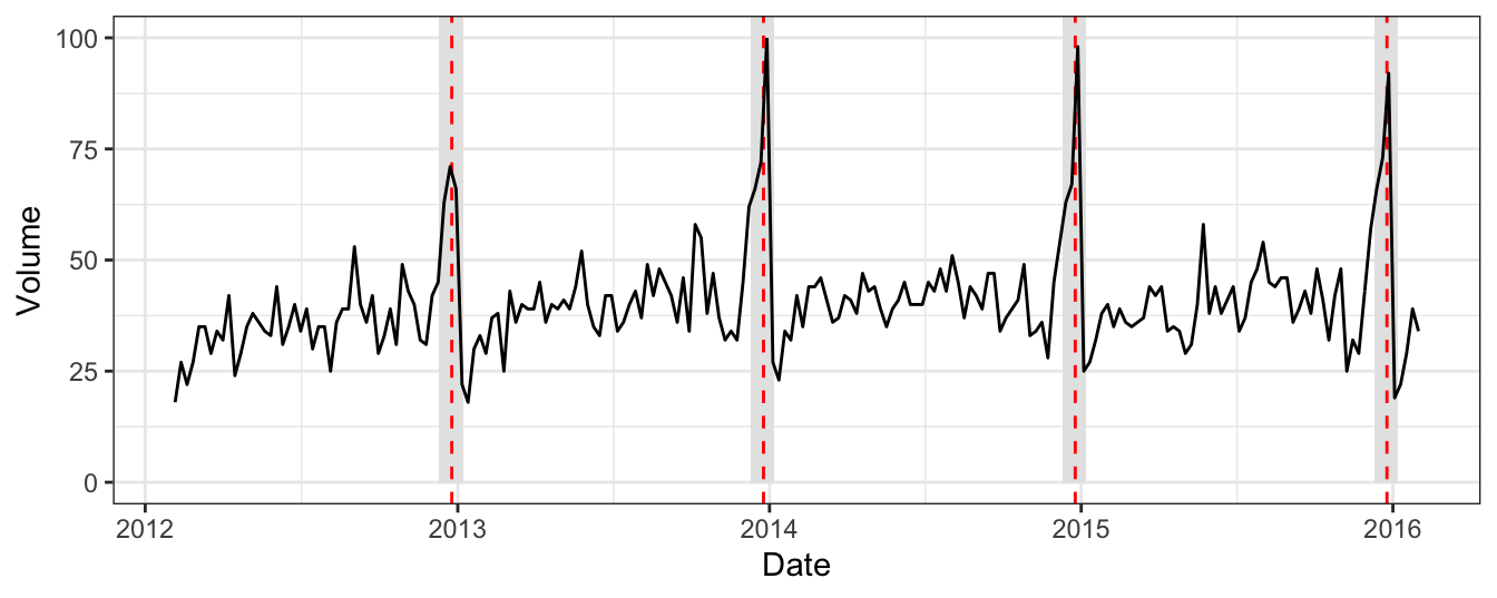
Figure 4.1: The hangover dataset. Google search traffic volume for the term hangover cure in the UK between Feb 2012 and Jan 2016. Red dashed lines highlight Christmas day each year and grey bars represent the region between 10 Dec and 7 Jan, classed as the holiday season each year.
Introducing the holiday period as a variable could be implemented in a number of ways. Here, we encode information about the holiday season as the variable holiday. If the given week is not in the holiday season, then this variable is 0, if part of the week is included then this is given by the appropriate proportion, and if the whole week if included in the holiday then the variable takes the value 1.
A simple linear regression to explore our aim is given by \[\begin{equation} V_i = \beta_0 + \beta_1 h_i + \epsilon_i, \end{equation}\] where \(V_i\) is the search traffic volume of week \(i\), \(h_i\) is the holiday season variable describing the proportion of week \(i\) that falls within the holiday period, and \(\epsilon_i\sim N(0,\sigma^2)\). The parameters of this model are interpreted as \(\beta_0\) being the average hangover search volume for weeks that are not during the holiday season and \(\beta_1\) is the average additional search traffic for a wholly holiday week. The proportional increase, or uplift as we will refer to it, is given by the ratio \(\frac{\beta_1}{\beta_0}\). The parameter \(\sigma^2\) describes the weekly variation in traffic volume, after the holiday season expected uplift has been accounted for.
4.1.2 Least squares fit
We’ll first fit the model using least squares. Even if the intention is to use a Bayesian approach, it can help to have some results obtained via another method for comparison.
ls_hang <- lm(volume ~ holiday, data = hangover)
summary(ls_hang)
##
## Call:
## lm(formula = volume ~ holiday, data = hangover)
##
## Residuals:
## Min 1Q Median 3Q Max
## -38.326 -3.988 0.806 5.012 31.070
##
## Coefficients:
## Estimate Std. Error t value Pr(>|t|)
## (Intercept) 37.988 0.624 60.88 <2e-16 ***
## holiday 30.942 2.344 13.20 <2e-16 ***
## ---
## Signif. codes: 0 '***' 0.001 '**' 0.01 '*' 0.05 '.' 0.1 ' ' 1
##
## Residual standard error: 8.616 on 207 degrees of freedom
## Multiple R-squared: 0.4571, Adjusted R-squared: 0.4544
## F-statistic: 174.3 on 1 and 207 DF, p-value: < 2.2e-16The least squares estimate would therefore lead to the estimate of the uplift being an 81.5% increase in search traffic during a week in the holiday season.
4.1.3 Bayesian approach in Stan
The most naive implementation of the hangover model in a Bayesian setting is to assume improper, flat priors for the three parameters, \(\lbrace \beta_0,\beta_1,\sigma^2\rbrace\). Under such an assumption, the .stan program code is given by:
data {
  int T ;
  vector[T] V ; // volume
  vector[T] h ; // holiday
}

parameters {
  real beta0 ;
  real beta1 ;
  real<lower = 0> sigma ;
}

model {
  V ~ normal(beta0 + beta1*h, sigma) ;
}

generated quantities {
  real uplift ;
  uplift = beta1 / beta0 ;
}
Note that we’ve used a generated quantities code block to monitor a quantify of interest that is a function of some parameters in the model:
\[uplift=\frac{\beta_1}{\beta_0}.\]
For each iteration of the sampler, the current samples of \(\beta_0\) and \(\beta_1\) are used to calculate a sample of the uplift. Generated quantities will appear in the parameter summary table. The ability to specify new variables as combinations of our parameters is extremely useful. In the likelihood approach above we can obtain a point estimate of the uplift, based on our maximum likelihood estimates, but quantifying the uncertainty of this is not so straightforward. But by specifying the uplift as a generated quantity, because it is calculated for each sampled pair of the two parameters, we can easily quantify uncertainty.
As in our previous examples, we use the following sample command to implement our HMC sampler. Here we have run two chains to demonstrate the output this produces (an overall summary and separate chain summaries). Each of the two chains ran for 1,000 iterations, with the first half removed as ‘burn-in’.
# set data in a way Stan understands
data <- list(T = nrow(hangover), V = hangover$volume, h = hangover$holiday)

sampling_iterations <- 1e4
fit_improper <- sampling(hangimproper,
                data = data,
                chains = 2,
                iter = sampling_iterations,
                warmup = sampling_iterations/2)
A summary of the results is given:
## $summary
##                mean      se_mean         sd         2.5%          50%
## beta0    37.9906300 0.0071924263 0.63568553   36.7381845   37.9871900
## beta1    30.9596242 0.0261558570 2.36568298   26.3229674   30.9711890
## sigma     8.6744835 0.0049039809 0.43725740    7.8678092    8.6550348
## uplift    0.8154774 0.0007847387 0.06775083    0.6836838    0.8156254
## lp__   -552.9759663 0.0176707715 1.25326271 -556.2108417 -552.6493043
##              97.5%    n_eff      Rhat
## beta0    39.223919 7811.489 0.9998941
## beta1    35.592301 8180.412 0.9998168
## sigma     9.586811 7950.177 0.9999100
## uplift    0.949653 7453.825 0.9998113
## lp__   -551.556051 5030.061 1.0001219
##
## $c_summary
## , , chains = chain:1
##
##          stats
## parameter         mean         sd         2.5%          50%        97.5%
##    beta0    37.9910379 0.63401834   36.7517638   37.9813528   39.2262303
##    beta1    30.9513961 2.32965854   26.3433769   30.9348518   35.5377681
##    sigma     8.6772193 0.43215957    7.8834217    8.6585727    9.5637623
##    uplift    0.8152383 0.06671415    0.6862336    0.8147219    0.9491596
##    lp__   -552.9514129 1.21760081 -556.0581414 -552.6439069 -551.5577478
##
## , , chains = chain:2
##
##          stats
## parameter         mean         sd         2.5%          50%       97.5%
##    beta0    37.9902221 0.63741151   36.7256590   37.9919937   39.221869
##    beta1    30.9678523 2.40137192   26.2721119   31.0061655   35.647604
##    sigma     8.6717477 0.44232280    7.8596864    8.6514699    9.611406
##    uplift    0.8157165 0.06877774    0.6811207    0.8169106    0.949670
##    lp__   -553.0005197 1.28759129 -556.3285699 -552.6606701 -551.554346
Note that the posterior means of \(\beta_0\) and \(\beta_1\) are similar to the least squares estimates.
The results of this implementation give a posterior mean for the uplift of 81.5% and a 95% credible interval of (68.4%, 95%).
4.2 Recap of logistic regression
You may have previously encountered generalised linear models (GLMs) in other courses and, in particular, that of logistic regression. Here we will give an overview of logistic regression as we are going to apply this to a more substantial modelling example in this chapter.
The simple linear regression model that you have encountered assumes that \[Y_i \sim N(\mu_i, \sigma^2),\] where \[\mu_i = \sum_{j=1}^m \beta_j X_{ij}.\]
Logistic regression is used when the dependent variable is not continuous, but is instead a binary variable (such as success and failure encoded as 1 and 0, respectively). The motivation behind this modelling approach is shown in Figure 4.2.
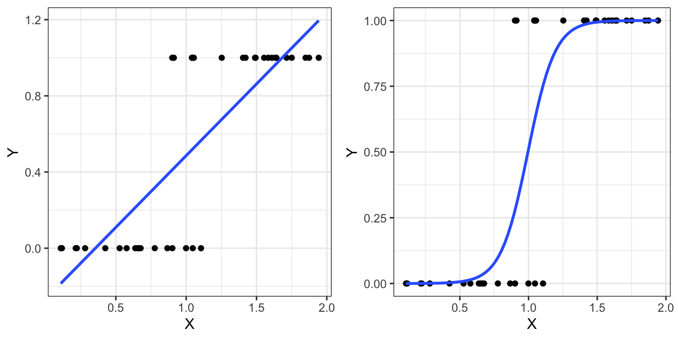
Figure 4.2: Motivation for using logistic regression. If our response variable is binary, simple linear regression (left) is problematic because predictions can exceed the (0,1) range. Alternatively, logistic regression (right) only produces predictions within the valid range.
To implement logistic regression we model the binary outcome as a Bernoulli response, \[Y_i \sim Bernoulli(\mu_i),\] where the probability of success is defined in terms of the explanatory variables as \[\mu_i=\P(Y_i=1)=\frac{e^{\sum_{j=1}^m \beta_j X_{ij}}}{1+e^{\sum_{j=1}^m \beta_j X_{ij}}}.\]
You can see that although we assume a different distribution for the response variable \(Y\) in logistic regression, we still retain a similar process of expressing the parameter of the distribution as a linear combination of the variables \(\lbrace X_j \rbrace\). The reason that the expression above differs to the expression for \(\mu\) in simple linear regression is because this now represents a probability and so is constrained between 0 and 1. Explicitly, we have applied a log-odds/logit transformation to \(\mu\), given by
\[\text{logit}(\mu) = \log \left( \frac{\mu}{1-\mu}\right),\]
and defined the regression model as
\[\text{logit}(\mu_i)=\sum_{j=1}^m \beta_j X_{ij}.\]
The most common method of estimating the \(\beta\) coefficients in a logistic regression model is based on maximum likelihood, using iteratively reweighted least squares. We will not cover the details of this during this course, but you may encounter this in your other courses. To implement model fitting in R, we use the glm package, where the glm function uses the syntax you are familiar with from implementing simple linear regression with lm.
4.3 Overview of mixed effects
A random effects model (or multilevel, hierarchical, mixed effects) is an extension to the regression theory you have previously met. In the simple linear regression model, a key assumption is that the observations \(Y_i\), for \(i=1,\ldots,n\) are independent from one another, with the joint distribution being \[\mathbf{Y}\sim N_n(\mathbf{X}\boldsymbol{\beta}, \sigma^2I_n),\] where \(I_n\) is the identity matrix. The vector of coefficients, \(\boldsymbol{\beta}\), is referred to as the coefficients of the fixed effects. The variation that we observe between the observations \(Y_i\) arises from the fixed structure defined by \(\mathbf{X}\boldsymbol{\beta}\) and the error associated with the shared variance \(\sigma^2\).
A common situation, however, is that observations arise in groups that are correlated, such as blocked group experiments or repeated measurements. The main idea of random effects models is recognising that the variables defining the grouping structure should be treated differently to how we would usually treat explanatory variables. We do this by introducing an additional source of variation that is group-specific. We can think of this as missing information on the groupings that, if it were available, would be included in the statistical model.
We can express a general mixed effects model as \[\mathbf{Y}=\mathbf{X}\boldsymbol{\beta}+\mathbf{Z}\boldsymbol{\gamma}+\boldsymbol{\epsilon},\] where:
- \(\mathbf{X}\boldsymbol{\beta}\) is defined as previously, with a design matrix \(\mathbf{X}\) based on independent variables, and a vector of coefficients that are to be estimated \(\boldsymbol{\beta}\),
- \(\mathbf{Z}\boldsymbol{\gamma}\) consists of another design matrix \(\mathbf{Z}\) that describes the grouping structure, and a vector of random effects \(\boldsymbol{\gamma}\sim N(\mathbf{0},G)\), and
- \(\boldsymbol{\epsilon}\sim N(\mathbf{0},\sigma^2I)\) is the error, as defined previously.
4.3.1 Simple example of a mixed effects model
Let’s consider a simple example. A set of observations correspond to repeated measures on the same group of subjects, so that we have observations \(Y_{ij}\) representing the \(j^\text{th}\) response from the \(i^\text{th}\) subject, for \(j=1,\ldots,k\) and \(i=1,\ldots,n\). Additionally we have observations of a single explanatory variable \(X_{ij}\) corresponding to the response. We could propose the model \[Y_{ij}=\beta_0+\beta_1X_{ij}+\gamma_i+\epsilon_{ij},\] so that there is a subject-specific random effect \(\gamma_i\sim N(0,\sigma_\gamma^2)\) that represents the assumption that observations from the same individual share some commonality, but that individuals differ from one another, having arisen from some common population that has a variation of \(\sigma_\gamma^2\). The within-group variation is then given by the residuals \(\epsilon_{ij}\sim N(0,\sigma^2)\). We note that, as we do not observe the random effects \(\gamma_i\), this random effects model has the following features:
- a general observation has the distribution \(Y_{ij}\sim N(\beta_0+\beta_1X_{ij},\sigma_\gamma^2+\sigma^2)\),
- observations from the same individual, say \(Y_{i1}\) and \(Y_{i2}\), have covariance \(\sigma_\gamma^2\), and
- observations from different individuals, say \(Y_{11}\) and \(Y_{32}\), are independent.
The above model differs from including a fixed effect that is a factor variable for the individual, with coefficient \(\gamma_i\). In that scenario the observations from the same individual would be uncorrelated. The results of model fitting would produce estimates of the effect of each subject in the experiment, but we would not have any information about the general population to predict anything about a new individual we have not seen.
4.3.2 Fixed or random effects?
This will depend on the aims of your analysis. If you’re interested in learning about the specific subjects/groups that you observed in your data, you want the fixed effects estimates of the groups. If you’re interested in learning about the general population that your subjects were sampled from, you want the random effect variation estimate. Statistical efficiency may also play a part in your decision making: if you have a large number of groups, then a fixed effects treatment involves many more parameters than the random effects counterpart.
4.4 Mixed effect logistic regression
In this section we will be using some experimental data to explore implementing mixed effect logistic regression. We are primarily interested in implementing this approach in a Bayesian framework, using Stan, but as a comparison we will also be implementing more traditional maximum likelihood approaches. As with any regression modeling application, we will be considering how the various independent variables that we have information on affect the dependent variable, which includes asking whether these variables have any significant effect upon the observed balance variable.
4.4.1 Balance experiment
The balance dataset, presented in Faraway (2016) contains the results of an experiments on the effects of surface and vision on balance. More details about the sources and an exploratory data analysis are available in these MAS61004 notes, but we will also perform an EDA here.
Balance was assessed qualitatively based on observation by the experimenter. This dependent variable, CTSIB, was on a four point ordinal scale, with 1 meaning ‘stable’ and 4 meaning ‘unstable’. Faraway converted this to a binary variable called Stable, where:
- 1 represents the original level 1 (stable), and
- 0 represents the original levels 2-4 (varying degrees of instability).
The balance of subjects were observed for:
Surface: two different surfaces (foam or normal), andVision: restricted and unrestricted vision (eyes closed, eyes open or with a dome placed over the head).
Forty subjects were studied (Subject), twenty males and twenty females (Sex), ranging in age from 18 to 38 (Age), with heights given in cm (Height) and weights in kg (Weight). Each subject was tested twice in each of the surface (two) and eye combinations (three), which results in a total of 12 measures per subject.
We will centre the Age, Height and Weight variables by subtracting the mean and dividing by the range. This can help with numerical computation, by weakening dependence between model parameters.
This study design is known as a full factorial design between subject, surface and vision with two replicates.
In addition to the observed dependent variables listed above, we also add a final variable (Dummy) which is an independent variable with no effect on the response. These are independent draws from a standard normal. We therefore have a variable that we know is not linked to the balance of individuals. This will be useful for considering whether other dependent variables display useful predictive information.
The data are constructed with the following code.
set.seed(123)
balance <- faraway::ctsib %>%
  mutate(Stable = ifelse(CTSIB == 1, 1, 0),
         Subject = factor(Subject),
         Age = (Age - mean(Age)) / diff(range(Age)),
         Weight = (Weight - mean(Weight)) / diff(range(Weight)),
         Height = (Height - mean(Height)) / diff(range(Height)),
         Dummy = round(rnorm(480), 1))
The full factorial experimental design/set-up is displayed in Table 4.2, which includes all observations for subject 1. The full data frame also contains the information on sex, age, height and weight for subject 1, along with that of the 39 other subjects. An extract of the data frame is shown in Table 4.3.
| Surface | Vision | CTSIB | Stable |
|---|---|---|---|
| norm | open | 1 | 1 |
| norm | open | 1 | 1 |
| norm | closed | 2 | 0 |
| norm | closed | 2 | 0 |
| norm | dome | 1 | 1 |
| norm | dome | 2 | 0 |
| foam | open | 2 | 0 |
| foam | open | 2 | 0 |
| foam | closed | 2 | 0 |
| foam | closed | 2 | 0 |
| foam | dome | 2 | 0 |
| foam | dome | 2 | 0 |
| Subject | Surface | Vision | Sex | Age | Height | Weight | Dummy | Stable |
|---|---|---|---|---|---|---|---|---|
| 1 | norm | open | male | -0.24 | 0.0822917 | -0.0506014 | -0.6 | 1 |
| 1 | norm | open | male | -0.24 | 0.0822917 | -0.0506014 | -0.2 | 1 |
| 1 | norm | closed | male | -0.24 | 0.0822917 | -0.0506014 | 1.6 | 0 |
| 1 | norm | closed | male | -0.24 | 0.0822917 | -0.0506014 | 0.1 | 0 |
| 1 | norm | dome | male | -0.24 | 0.0822917 | -0.0506014 | 0.1 | 1 |
| 1 | norm | dome | male | -0.24 | 0.0822917 | -0.0506014 | 1.7 | 0 |
The response variable for this experiment is binary, as we have stable or unstable observations. It is therefore sensible to model this using logistic regression. This is our first modelling decision.
There are multiple explanatory variables that could be incorporated in such a model, and these could feature as fixed or random effects. Determining the appropriateness of variables as fixed or random effects is an important skill. In the following we carry out some exploratory data analysis to explore the appropriateness of some modelling decisions we could implement. For clarity, we will refer to the variables as:
SurfaceandVisionas design variables. Note that these are both factor variables.Sex,Age,Height,Weightas covariates. Note thatSexis a factor variable.Subjectas the grouping variable. Note that this is a factor variable.
4.4.2 Exploratory data analysis
4.4.2.1 Considering the grouping variable as a fixed or random effect
Let’s consider the variable Subject, which is a factor variable of which we have observed 40 categories of. By applying logistic regression we are modeling the probability of stability, given some combination of observed variables. If a given subject was only ever observed to give the same outcome (say all unstable) then this would cause problems if Subject was included as a fixed effect term, because the probability of stability would be 0 for that subject. For any data application you are working on, this is an important aspect of your data that you should check in the exploratory analysis stage.
Considering the balance data, we can compute the proportion of stable outcomes for the 12 observations of each subject, and tabulate how many subjects have each possible proportion. This is given in Table 4.4. From this we see that five subjects were unstable for all observations. We therefore cannot include a subject-specific fixed effect in our model for this experiment. If we would like to incorporate the concept of correlation between repeated measurements on the same subject, we can make a decision to include subject as a random effect.
| propStable | n |
|---|---|
| 0.0000000 | 5 |
| 0.0833333 | 4 |
| 0.1666667 | 15 |
| 0.2500000 | 3 |
| 0.3333333 | 4 |
| 0.4166667 | 3 |
| 0.5000000 | 4 |
| 0.6666667 | 2 |
4.4.2.2 Considering the design variables effect
Another set of factor variables we would be interested in including in our balance model are the Surface and Vision variables, with two and three categories, respectively. These were the experimental design variables and so are of particular importance in determining their effect on balance.
We produce contingency tables for number of observations that were stable/unstable at the different levels of the design variables:
##       Surface
## Stable foam norm
##      0  230  136
##      1   10  104
## Vision
## Stable closed dome open
## 0 143 138 85
## 1 17 22 75This shows that there is a mixture of stability observations for the two categories of surface, and similarly for the three categories of vision. These contingency tables also highlight that there does appear to be an effect on balance between the categories. We could consider including both Surface and Vision are fixed effects in our regression.
Note, however, if we look at the combinations of these variables together we see in Table 4.5 the proportions of stability. Here we see that two combinations of surface and vision were only ever observed to be unstable. We therefore would find complications if we attempt to include a fixed effects interaction term between Surface and Vision. Our initial model will therefore feature both the design variables as fixed effects, but will not feature the possible interaction term.
| Surface | Vision | propStable |
|---|---|---|
| foam | closed | 0.0000 |
| foam | dome | 0.0000 |
| foam | open | 0.1250 |
| norm | closed | 0.2125 |
| norm | dome | 0.2750 |
| norm | open | 0.8125 |
4.4.2.3 Considering the covariates
The remaining variables in our data are the covariates Sex, Age, Height, Weight, and our dummy variable Dummy. Before deciding on our proposed regression model, we can produce exploratory plots of whether the probability of stability is affected by each variable. This exploratory analysis is important, because it could highlight important issues with our observations that were otherwise would not be aware of. It may also be the case that we have a very large number of covariates in an application, and including all of them in a model may not be appropriate.
In Figure 4.3, we have calculated the proportion of stable observations for each subject, and plotted this against Sex. This suggests that this variable has some affect on stability and would be an appropriate fixed effect choice for inclusion in our model. Remember that our fitted model may still indicate that this effect is not significant.
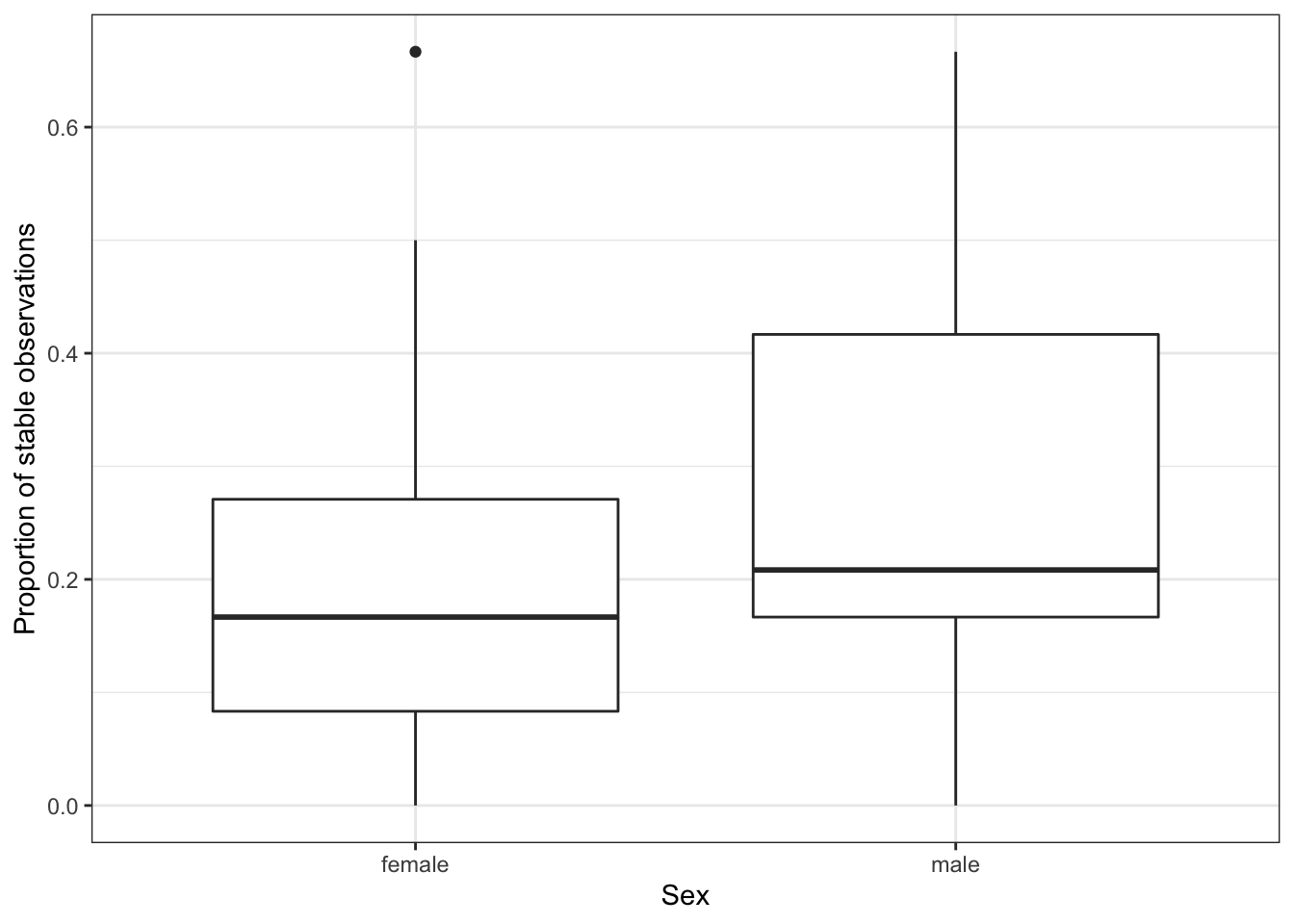
Figure 4.3: The proportion of stable observations out of the 12 carried out for each subject, split by the sex variable.
In Figure 4.4, we have plotted the age, weight, height and dummy variables, split by sex and stability. These plots are useful for considering the effects of these four covariates on stability, but also their interaction with the sex covariate. We can see that there is a fairly clear separation between the two sexes in terms of the height and weight of individuals (males are taller and heavier). Let’s explore this a little more with pairs plots in Figure 4.5. The separation of the two sexes is obvious, as is the high correlation between height and weight. This structure in the data is useful to be aware of, and suggests that it may not be necessary (or even useful) to include both height and weight as variables in our model.
When considering the possible effects of the covariates on stability in Figure 4.4 it is useful to have our dummy variable. We know that this variable is independent of stability, and so when comparing the stable/unstable box plot distributions we see patterns that can only have arisen by chance. This provides some perspective for considering whether the remaining three covariates in this plot also display differences in stability through random chance or an actual effect. These plots suggest that age, weight and height may not be at all important in determining stability.
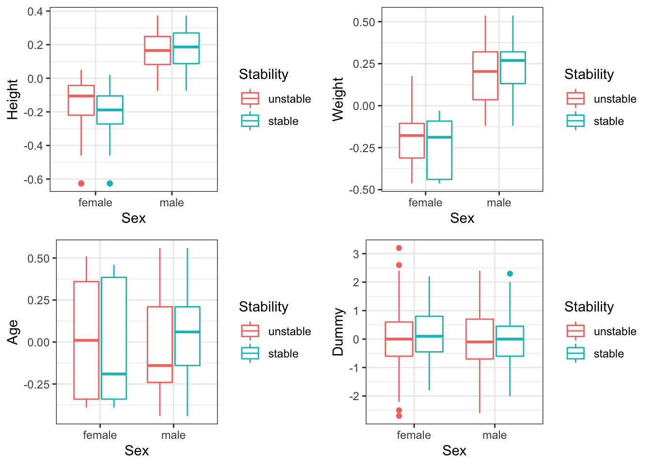
Figure 4.4: The height/weight/age/dummy variable of individuals split by sex and stability.
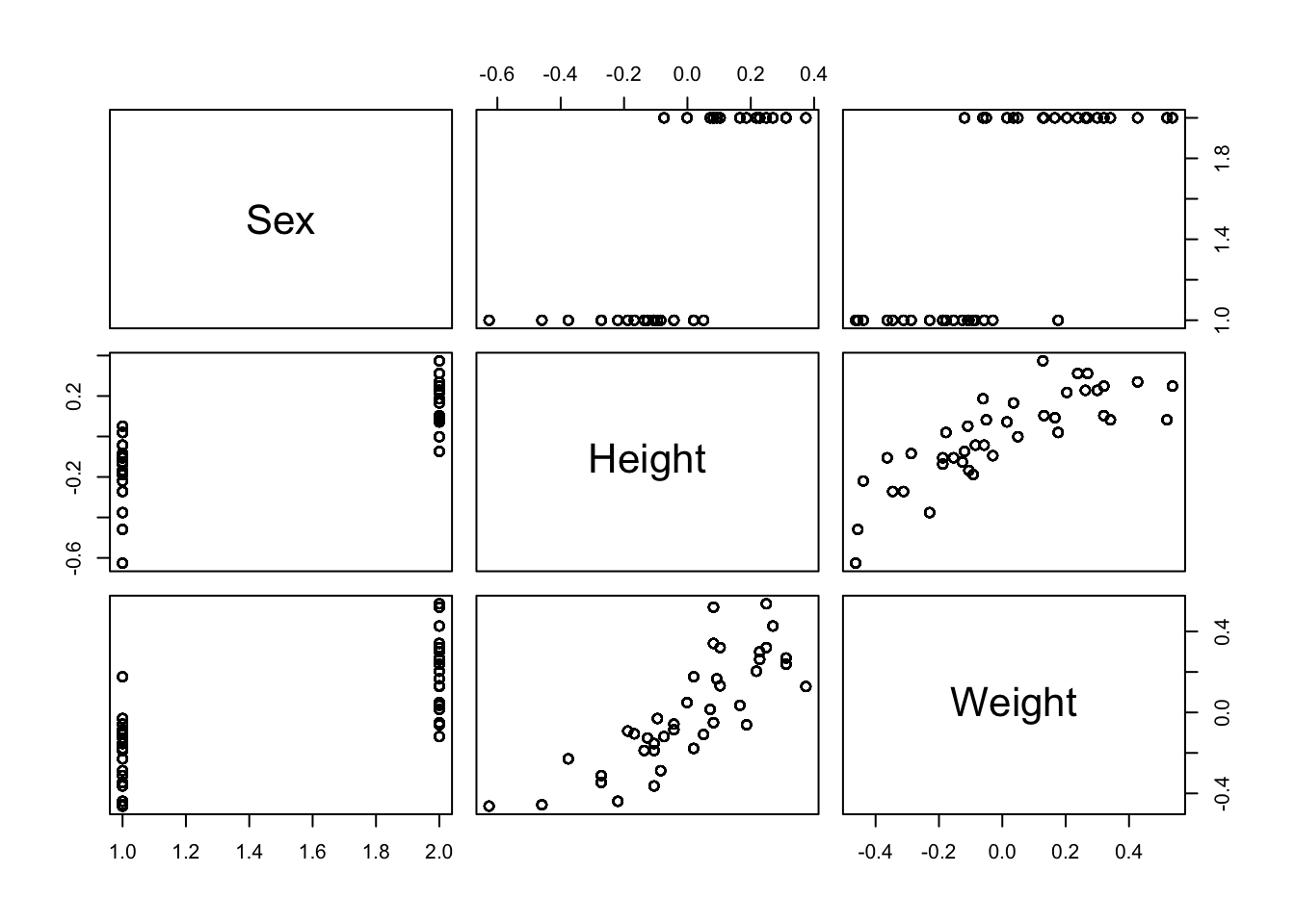
Figure 4.5: The combinations of sex, height and weight variables for the balance experiment.
4.4.3 Maximum likelihood approach
4.4.3.1 Ordinary logistic regression (no grouping variable)
In the above we found that we cannot include Subject as a fixed effect for this experiment. We would like to include Subject as a random effect to take into account the variability between individuals. However, first for simplicity, we will implement the model without this feature. We are therefore modeling stability as a logistic regression, with fixed effects for the design variables and the covariates. Let’s set this up with formal notation.
Define \(Y_{ijkl}\) to be the stability response for subject \(i=1,\ldots,12\), surface \(j=1,2\), vision setting \(k=1,2,3\), and replicate \(l=1,2\). We have \[Y_{ijkl} \sim Bernoulli(\mu_{ijkl}),\] and we suppose \[\text{logit}(\mu_{ijkl}) = \beta_0 + \alpha_j + \gamma_k + \beta_1 x_{1,i} + \beta_2 x_{2,i} + \beta_3 x_{3,i} + \beta_4 x_{4,i} + \beta_5 x_{5,ijkl},\] where
- \(\alpha_j\) is the additive contribution of the surface factor, with \(\alpha_1=0\),
- \(\gamma_k\) is the additive contribution of the vision factor, with \(\gamma_1=0\),
- \(\beta_1\) is the additive contribution of the sex factor where \(x_{1, i}\) is the sex of subject \(i\), with \(x_{1, i}=1\) for a male and 0 for a female,
- \(x_{2,i}, x_{3,i}, x_{4,i}\) are the corresponding age, height, weight covariates of subject \(i\), and
- \(x_{5,ijkl}\) is the dummy variable.
Note that we have not included the subject as an effect here, and that the subscript \(i\) is needed only to identify the subject’s covariate values.
Exercise:
Spend some time making sure you understand the interpretation of the coefficients in this model definition. For example, what is the significance of \(\beta_0\)? Or what combination of coefficients produces the expected probability of stability for a 20 year old female with restricted vision?
Our glm model definition and summary is given here:
glmNoSubject <-
  glm(Stable ~ Surface + Vision +
        Sex +
        Age + Height + Weight + Dummy,
      family = binomial,
      data = balance)

summary(glmNoSubject)
##
## Call:
## glm(formula = Stable ~ Surface + Vision + Sex + Age + Height +
## Weight + Dummy, family = binomial, data = balance)
##
## Deviance Residuals:
## Min 1Q Median 3Q Max
## -2.41266 -0.51936 -0.13654 -0.04721 2.62161
##
## Coefficients:
## Estimate Std. Error z value Pr(>|z|)
## (Intercept) -6.29989 0.65959 -9.551 < 2e-16 ***
## Surfacenorm 4.05639 0.45701 8.876 < 2e-16 ***
## Visiondome 0.38653 0.38537 1.003 0.315851
## Visionopen 3.26062 0.42425 7.686 1.52e-14 ***
## Sexmale 1.46294 0.52152 2.805 0.005029 **
## Age 0.07167 0.48681 0.147 0.882950
## Height -4.86326 1.31178 -3.707 0.000209 ***
## Weight 2.71654 1.05972 2.563 0.010364 *
## Dummy 0.28974 0.16266 1.781 0.074881 .
## ---
## Signif. codes: 0 '***' 0.001 '**' 0.01 '*' 0.05 '.' 0.1 ' ' 1
##
## (Dispersion parameter for binomial family taken to be 1)
##
## Null deviance: 526.25 on 479 degrees of freedom
## Residual deviance: 291.96 on 471 degrees of freedom
## AIC: 309.96
##
## Number of Fisher Scoring iterations: 6Exercise:
Spend some time interpreting this model output. What do these results indicate about the three levels of the Vision variable? Do these results agree with your understanding of the data given our exploratory data analysis? What conclusions would you report in a summary to a client if you were analysing this data for them?
4.4.3.2 Random effects (including the grouping variable)
Will will extend the previous model to include a random effect for each of the 12 different subjects.
The full model is now \[\text{logit}(\mu_{ijkl}) = \beta_0 + \alpha_j + \gamma_k + \beta_1 x_{1,i} + \beta_2 x_{2,i} + \beta_3 x_{3,i} + \beta_4 x_{4,i} + \beta_5 x_{5,ijkl} + b_i,\] with the extra random effects term \(b_i \sim N(0,\sigma^2_b)\).
Let’s fit this random effects GLM with the lme4 package:
glmSubjectRandom <-
  lme4::glmer(Stable ~ Surface + Vision +
                Sex +
                Age + Height + Weight + Dummy +
                (1 | Subject),
              family = binomial,
              data = balance,
              nAGQ = 25)
## Warning in checkConv(attr(opt, "derivs"), opt$par, ctrl = control$checkConv, :
## Model failed to converge with max|grad| = 0.320305 (tol = 0.002, component 1)We get a message that the method for model fitting failed to converge! It’s important to remember that there is not a closed form expression for the maximum likelihood estimates in mixed effects generalised linear models, and numerical methods must be used. This means that a solution is not always viable.
Let’s return to our exploratory data analysis, and recall how we suspected little information was being gained by our collection of covariates, and in particular, that height and weight were highly correlated. So we’re going to proceed by removing the Height variable.
glmSubjectRandom <-
  lme4::glmer(Stable ~ Surface + Vision +
                Sex +
                Age + Weight + Dummy +
                (1 | Subject),
              family = binomial,
              data = balance,
              nAGQ = 25)

summary(glmSubjectRandom)
## Generalized linear mixed model fit by maximum likelihood (Adaptive
## Gauss-Hermite Quadrature, nAGQ = 25) [glmerMod]
## Family: binomial ( logit )
## Formula: Stable ~ Surface + Vision + Sex + Age + Weight + Dummy + (1 |
## Subject)
## Data: balance
##
## AIC BIC logLik deviance df.resid
## 251.2 288.8 -116.6 233.2 471
##
## Scaled residuals:
## Min 1Q Median 3Q Max
## -4.9493 -0.1411 -0.0196 -0.0007 5.6453
##
## Random effects:
## Groups Name Variance Std.Dev.
## Subject (Intercept) 8.491 2.914
## Number of obs: 480, groups: Subject, 40
##
## Fixed effects:
## Estimate Std. Error z value Pr(>|z|)
## (Intercept) -11.20462 1.87176 -5.986 2.15e-09 ***
## Surfacenorm 7.32839 1.07053 6.846 7.62e-12 ***
## Visiondome 0.67763 0.52966 1.279 0.201
## Visionopen 6.14100 0.99263 6.187 6.15e-10 ***
## Sexmale 1.89216 1.64924 1.147 0.251
## Age 0.05018 1.63334 0.031 0.975
## Weight -0.05908 3.03973 -0.019 0.984
## Dummy 0.23971 0.23094 1.038 0.299
## ---
## Signif. codes: 0 '***' 0.001 '**' 0.01 '*' 0.05 '.' 0.1 ' ' 1
##
## Correlation of Fixed Effects:
## (Intr) Srfcnr Visndm Visnpn Sexmal Age Weight
## Surfacenorm -0.821
## Visiondome -0.246 0.109
## Visionopen -0.809 0.831 0.377
## Sexmale -0.591 0.174 0.023 0.184
## Age -0.058 0.002 0.003 0.006 0.131
## Weight 0.366 -0.028 -0.003 -0.039 -0.765 -0.172
## Dummy -0.014 -0.012 0.006 0.007 0.027 0.014 0.007This has helped and convergence has been reached.
Exercise: How do the fitted estimates compare to the fitted model that did not consider a subject random effect?
The summary of this fitted model suggests that the covariates are not significantly useful in explaining the variation in our data. So we can explore the possibility of removing these (the sex, age, height, weight, and of course the dummy variable we know for certain is uninformative). This reduced model is fit as in the below, and the nested model comparison shows that indeed, we could reasonably drop the subject covariate information.
glmSubjectRandomReduced <-
  lme4::glmer(Stable ~ Surface + Vision +
                (1 | Subject),
              family = binomial,
              data = balance)

anova(glmSubjectRandomReduced,
      glmSubjectRandom)
## Data: balance
## Models:
## glmSubjectRandomReduced: Stable ~ Surface + Vision + (1 | Subject)
## glmSubjectRandom: Stable ~ Surface + Vision + Sex + Age + Weight + Dummy + (1 | Subject)
## npar AIC BIC logLik deviance Chisq Df
## glmSubjectRandomReduced 5 246.40 267.26 -118.20 236.40
## glmSubjectRandom 9 251.23 288.79 -116.61 233.23 3.1682 4
## Pr(>Chisq)
## glmSubjectRandomReduced
## glmSubjectRandom 0.5301Let’s summarise this reduced model:
summary(glmSubjectRandomReduced)## Generalized linear mixed model fit by maximum likelihood (Laplace
## Approximation) [glmerMod]
## Family: binomial ( logit )
## Formula: Stable ~ Surface + Vision + (1 | Subject)
## Data: balance
##
## AIC BIC logLik deviance df.resid
## 246.4 267.3 -118.2 236.4 475
##
## Scaled residuals:
## Min 1Q Median 3Q Max
## -4.2407 -0.1570 -0.0160 -0.0004 6.3710
##
## Random effects:
## Groups Name Variance Std.Dev.
## Subject (Intercept) 11.2 3.346
## Number of obs: 480, groups: Subject, 40
##
## Fixed effects:
## Estimate Std. Error z value Pr(>|z|)
## (Intercept) -10.9807 1.9061 -5.761 8.37e-09 ***
## Surfacenorm 7.8425 1.3011 6.027 1.67e-09 ***
## Visiondome 0.6904 0.5344 1.292 0.196
## Visionopen 6.5930 1.2099 5.449 5.05e-08 ***
## ---
## Signif. codes: 0 '***' 0.001 '**' 0.01 '*' 0.05 '.' 0.1 ' ' 1
##
## Correlation of Fixed Effects:
## (Intr) Srfcnr Visndm
## Surfacenorm -0.930
## Visiondome -0.259 0.116
## Visionopen -0.918 0.882 0.3364.4.4 Bayesian approach using Stan
We’re going to define our mixed effects GLM in Stan using the building blocks that we have previously used. The following .stan program defines our model, and we will explain each of the blocks contained here in the following.
data {
  // number of observations
  int<lower = 0> Nobs ;
  // number of random effects groups (40 subjects)
  int<lower = 0> Nsubs ;
  // number of independent variables
  int<lower = 0> Npreds ;
  // the observations, note that they are a vector of binary outcomes
  int<lower = 0, upper = 1> y[Nobs] ;
  // vector associating each observation with its corresponding subject
  int<lower = 1, upper = Nsubs> subject[Nobs] ;
  // the independent variables
  matrix[Nobs, Npreds] X ;
}

parameters {
  vector[Nsubs] b ;
  real<lower = 0> sigmab ;
  vector[Npreds] beta ;
}

model {
  b ~ normal(0, sigmab) ;
  sigmab ~ cauchy(0, 1) ;
  for(n in 1:Nobs) {
    y[n] ~ bernoulli_logit(X[n] * beta + b[subject[n]]) ;
  }
}

generated quantities {
  real bTilde = normal_rng(0, sigmab) ;
  int<lower = 0, upper = 1> yTilde = bernoulli_logit_rng(X[1] * beta + bTilde) ;

}
4.4.4.1 The data block
Remember that the data block specifies the information that we observe. Previously in our hangover example, this involved the dependent variable and the single independent variable. Here we have the same process, but because we have multiple independent variables, we must combine these into a design matrix. Let’s discuss the structure of this matrix in more detail.
If the observations are collected in a vector \(\mathbf{Y}\), with mean vector \(\boldsymbol{\mu}\), we have
\[\boldsymbol{\mu} = X\boldsymbol{\beta} + Z\mathbf{b},\]
with \(\mathbf{b}\) the vector of random effects. When we use functions such as glmer, the function will implicitly have been creating our design matrix for us from the model definition we provide. This is actually stored as part of the results of the fitted model, so we can use the command model.matrix to extract the design matrix \(X\) from the models we have already implemented. Here we’ll implement the model equivalent to glmSubjectRandom from earlier, and this shows an extract of the design matrix:
##   (Intercept) Surfacenorm Visiondome Visionopen Sexmale   Age      Weight Dummy
## 1           1           1          0          1       1 -0.24 -0.05060137  -0.6
## 2           1           1          0          1       1 -0.24 -0.05060137  -0.2
## 3           1           1          0          0       1 -0.24 -0.05060137   1.6
## 4           1           1          0          0       1 -0.24 -0.05060137   0.1
## 5           1           1          1          0       1 -0.24 -0.05060137   0.1
## 6           1           1          1          0       1 -0.24 -0.05060137   1.7
4.4.4.2 The parameter block
In our simple hangover regression, we had three parameters: the intercept, slope and error variance. We specified these as three separate continuous variables. In this more complex case we do not need to create a long list of parameters, but can instead use vectors. We declare as parameters:
sigmab: the standard deviation \(\sigma_b\) in the random effects distribution \(b_i \sim N(0,\sigma^2_b)\),beta: the coefficients \(\boldsymbol{\beta}\) for all the fixed effects. Note in our notation above this is the collection \(\lbrace \alpha_2,\gamma_2, \gamma_3, \beta_0, \beta_1, \beta_2, \beta_4, \beta_5 \rbrace\) (remember, we have removed \(\beta_3\) as this is the height coefficient), andb: the random effects themselves.
4.4.4.3 The model block
Our random effects GLM definition consists of:
- The random effects that are normally distributed with zero mean, i.e. \(b_i \sim N(0,\sigma_b^2)\) for \(i=1,\ldots,40\).
- A prior distribution for the random effect variation, \(\sigma_b \sim Cauchy(0,1)\).
- The distribution of the response variable, which is Bernoulli, but with the logit link equation \(\log (\frac{\mu}{1-\mu})\), i.e. \(Y_j \sim Bernoulli (\mu_j)\) where \(\text{logit}(\mu_j)=X_j\boldsymbol{\beta}+b_i\) for \(j=1,\ldots,480\) and \(i\) is the subject corresponding to observation \(j\).
- A prior distribution for the vector coefficients, \(\boldsymbol{\beta}\). By leaving out this specification, Stan will assume an improper uniform prior, i.e. \(f(\beta_l)\propto 1\) for the \(l=1,\ldots,8\) as we have a set of 8 independent variables in our chosen model.
Some detail on the choice of the prior for \(\sigma_b\). A suggestion (in Faraway) is to use a ‘half-Cauchy’, truncated at 0. This half-Cauchy distribution is given by
\[f(\sigma_b) = 2\frac{1}{\pi (1 + \sigma_b^2)},\]
for \(\sigma_b >0\), and \(f(\sigma_b) = 0\) otherwise. To set this up in Stan, we specify sigmab as a real-valued parameter with lower bound 0, and then separately, give it a Cauchy distribution in the model block.
It’s important to question our prior choices we make and whether the impact they have on our posterior is appropriate. The definition of the prior we have used involves \(v=1\), and has prior median for \(\sigma_b\) equal to 1. The 99th percentile of the prior is 64, which is implausibly large. We will return to this when we analyse our posterior results and consider whether this was appropriate.
4.4.4.4 The generated quantities block
As we are building up our experience with using Stan, we will now introduce the generated quantities block. We can get Stan to sample directly from the posterior predictive distribution, and this is the most common use of the generated_quantities block. We’ll consider a new subject, with design and covariate values \(\tilde{x}\) which are equal to the first observation (i.e. the first row of the design matrix):
## (Intercept) Surfacenorm  Visiondome  Visionopen     Sexmale         Age
##        1.00        1.00        0.00        1.00        1.00       -0.24
##      Weight       Dummy
##       -0.05       -0.60
Let \(\tilde{Y}\) be the observed response for this new subject. We want to sample from the distribution \(\P(\tilde{Y}|Y, X, \tilde{x})\): we do so via \[\P(\tilde{Y}|Y, X, \tilde{x}) =\int \P(\tilde{Y}|\tilde{b}, \tilde{x},\beta)f(\tilde{b}|\sigma_b)f(\sigma_b, \beta|Y, X)d\tilde{b}d\sigma_b d\beta,\] where \(\tilde{b}\) is the random effect for the new subject. Hence we need to get Stan to sample \(\tilde{b}\), and then sample \(\tilde{Y}\) given the current sampled value of the parameters \(\beta, \sigma_b\). Notice that we therefore do not predict the response of a new individual only as the contribution from the fixed effects (i.e. the expected value \(\mathbf{X}\boldsymbol{\beta}\)), but we sample a subject random effect to add to this fixed effects value and then sample from the binomial distribution with such an expected value.
4.4.4.5 Sampling and output
As with previous examples, we group our data into the list form that Stan requires, and use the sampling function to implement the HMC algorithm:
glmData <- list(Nobs = nrow(balance),
                Nsubs = length(unique(balance$Subject)),
                Npreds = ncol(designMatrix),
                y = balance$Stable,
                subject = as.numeric(balance$Subject),
                X = designMatrix)

myfit <- sampling(glmRandomEffects,
                  data = glmData,
                  cores = 7,
                  refresh = 0)
Let’s explore the output from our fitted model in Stan. We can print out a summary of our results, as previously, and explore the trace-plots for convergence. Note that the summary print-out includes:
- the subject random effects variance, \(\sigma_b^2\),
- the fixed effects coefficients \(\boldsymbol{\beta}\),
- all 40 of the subject-specific random effects themselves, \(b_1,\ldots,b_{40}\),
- the samples from the posterior predictive distribution, \(\tilde{b},\tilde{Y}\), and
- the Hamiltonian energy itself.
In reality, we are probably not interested in the actual random effects, so we will omit these from the results plots in the following.
## Inference for Stan model: c808de51faf75c5c13f75aad1c4debdc.
## 4 chains, each with iter=2000; warmup=1000; thin=1;
## post-warmup draws per chain=1000, total post-warmup draws=4000.
##
##            mean se_mean   sd    2.5%     50%   97.5% n_eff Rhat
## b[1]       0.02    0.04 1.69   -3.32    0.02    3.32  1550    1
## b[2]      -1.76    0.05 1.91   -5.70   -1.72    1.78  1793    1
## b[3]      -6.40    0.07 2.44  -11.90   -6.10   -2.37  1079    1
## b[4]      -4.12    0.05 2.01   -8.56   -3.99   -0.47  1349    1
## b[5]      -2.16    0.04 1.91   -6.07   -2.13    1.44  2044    1
## b[6]       2.36    0.04 1.56   -0.59    2.34    5.51  1330    1
## b[7]      -1.60    0.04 1.78   -5.18   -1.50    1.72  2338    1
## b[8]      -0.03    0.04 1.91   -3.72   -0.01    3.62  2300    1
## b[9]      -0.01    0.03 1.82   -3.70    0.02    3.55  3642    1
## b[10]      1.41    0.03 1.40   -1.32    1.42    4.11  1714    1
## b[11]     -1.56    0.04 1.79   -5.19   -1.51    1.77  2237    1
## b[12]     -1.59    0.04 1.84   -5.51   -1.53    1.86  2280    1
## b[13]     -1.53    0.04 1.88   -5.33   -1.49    1.99  1882    1
## b[14]     -5.11    0.06 2.56  -11.14   -4.78   -1.06  1587    1
## b[15]      0.05    0.03 1.77   -3.38    0.06    3.49  3619    1
## b[16]      4.24    0.05 1.72    1.01    4.18    7.83  1344    1
## b[17]      3.22    0.04 1.59    0.23    3.15    6.48  1390    1
## b[18]      0.21    0.04 1.88   -3.45    0.20    3.89  2188    1
## b[19]      0.33    0.04 1.69   -3.15    0.37    3.59  1715    1
## b[20]      1.20    0.05 1.75   -2.19    1.19    4.69  1282    1
## b[21]      3.50    0.06 1.86    0.13    3.38    7.42   957    1
## b[22]     -2.24    0.04 1.92   -6.21   -2.20    1.50  2021    1
## b[23]     -1.61    0.05 2.17   -5.95   -1.55    2.61  2037    1
## b[24]     -1.63    0.04 1.80   -5.38   -1.56    1.71  2299    1
## b[25]      5.54    0.05 1.82    2.35    5.42    9.44  1406    1
## b[26]      3.45    0.05 1.75    0.24    3.39    7.20  1267    1
## b[27]      7.50    0.07 2.05    4.07    7.31   12.02   980    1
## b[28]     -0.01    0.04 1.93   -3.76   -0.01    3.81  2355    1
## b[29]      4.83    0.05 1.91    1.39    4.73    8.96  1292    1
## b[30]     -4.84    0.06 2.41  -10.30   -4.57   -0.89  1595    1
## b[31]      2.29    0.05 1.81   -1.15    2.22    6.09  1305    1
## b[32]      2.29    0.04 1.62   -0.88    2.28    5.42  1550    1
## b[33]      3.37    0.05 1.70    0.25    3.29    6.81  1329    1
## b[34]     -1.63    0.04 1.84   -5.47   -1.56    1.74  2301    1
## b[35]      3.31    0.04 1.44    0.63    3.29    6.31  1441    1
## b[36]      0.10    0.04 1.95   -3.81    0.11    3.91  2600    1
## b[37]     -4.93    0.07 2.53  -10.93   -4.65   -0.77  1479    1
## b[38]     -4.73    0.07 2.57  -10.68   -4.54   -0.20  1541    1
## b[39]      0.22    0.04 1.91   -3.42    0.21    3.99  2251    1
## b[40]     -2.22    0.04 1.87   -6.08   -2.17    1.39  2230    1
## sigmab     3.63    0.03 0.79    2.39    3.54    5.44   660    1
## beta[1]  -12.98    0.09 2.34  -18.40  -12.72   -9.09   621    1
## beta[2]    8.38    0.05 1.30    6.18    8.26   11.36   678    1
## beta[3]    0.75    0.01 0.55   -0.28    0.75    1.84  3526    1
## beta[4]    7.08    0.05 1.24    5.03    6.96   10.00   651    1
## beta[5]    2.43    0.07 2.08   -1.30    2.30    6.81   886    1
## beta[6]    0.12    0.06 2.12   -4.14    0.13    4.16  1234    1
## beta[7]   -0.62    0.12 3.76   -8.15   -0.60    6.39  1047    1
## beta[8]    0.24    0.00 0.25   -0.25    0.24    0.72  4292    1
## bTilde    -0.04    0.06 3.79   -7.44   -0.05    7.65  3693    1
## yTilde     0.86    0.01 0.35    0.00    1.00    1.00  3667    1
## lp__    -154.44    0.28 7.12 -169.55 -154.05 -141.87   654    1
##
## Samples were drawn using NUTS(diag_e) at Sun Mar 20 17:05:22 2022.
## For each parameter, n_eff is a crude measure of effective sample size,
## and Rhat is the potential scale reduction factor on split chains (at
## convergence, Rhat=1).
The trace plots of the four chains (only showing the samples after the burn-in period) are given in Figure 4.6. This shows the \(\sigma_b^2\) parameter and the fixed effects coefficients \(\boldsymbol{\beta}\), but re-labelled to add some descriptive context to the interpretation of each.
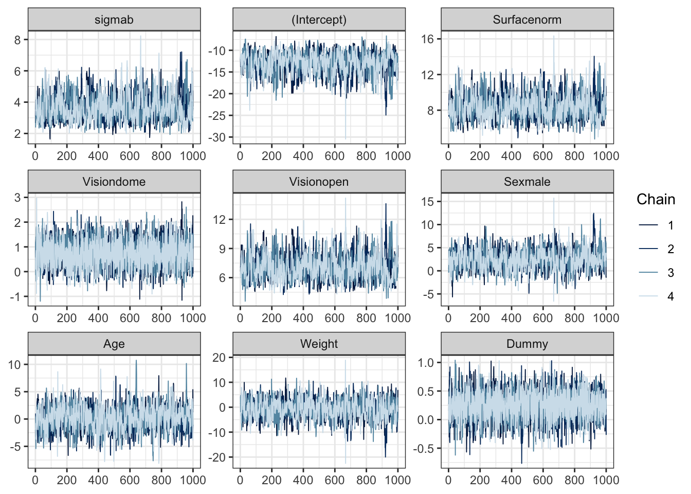
Figure 4.6: Trace plots of the sampled parameters for the balance experiment, fitting a random effects GLM in Stan. Note that the beta parameters have been relabelled here descriptively to add context.
Posterior credible intervals are shown for these parameters in Figure 4.7. Again, the parameters have been relabelled to add some descriptive context to each.
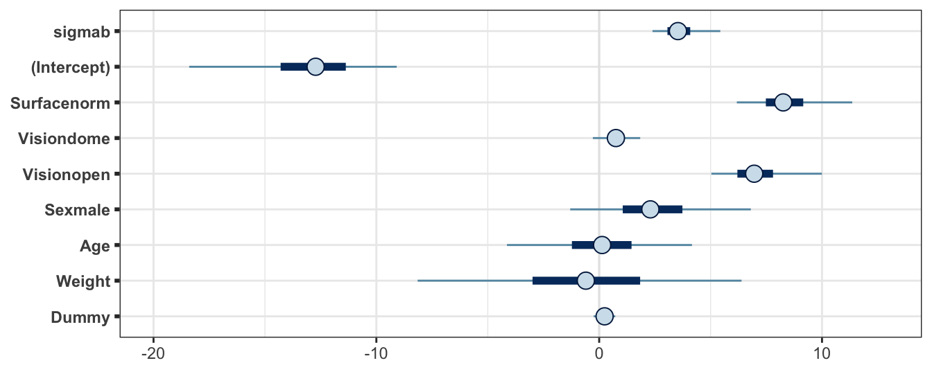
Figure 4.7: Posterior credible interval summaries for the balance experiment, fitting a random effects GLM in Stan. Note that the beta parameters have been relabelled here descriptively to add context. Point gives the posterior median, bar gives the interval with quantiles at 0.25 and 0.75, and the line gives the quantiles at 0.025 and 0.975.
Exercise
What information can we determine from these plots?
Are you satisfied about the convergence of the HMC sampler? What other diagnostics could you explore?
What do the posterior credible intervals suggest about our full proposed model?
4.4.4.6 Examining the effect of our choice of prior
We will look more carefully at \(\sigma_b\), the subject random effect. Recall that this was the only parameter we set a ‘proper’ prior for, using a half-Cauchy, and it featured a heavy right tail. It’s important to check that our posterior is not just a reflection of our prior, and that there truly is information from that data here.
We compare the prior and posterior tails for \(\sigma_b\) in Table 4.6. We see that the data does seem to have pulled in the posterior; both away from the heavy tail, and away from the prior median. To explore this visually, Figure 4.8 shows the prior density for \(\sigma_b\) (black line), along with a histogram of the posterior samples (blue) and the estimate of \(\sigma_b\) from the likelihood-based approach using lme4 that we implemented earlier. Note that lme4 does not give error estimates of random effect parameters, so we would have nothing more than this point estimate were we using the maximum likelihood approach.
| Prior | Posterior | |
|---|---|---|
| 1% | 0.016 | 2.2 |
| 5% | 0.079 | 2.5 |
| 50% | 1.000 | 3.5 |
| 95% | 13.000 | 5.1 |
| 99% | 64.000 | 6.0 |
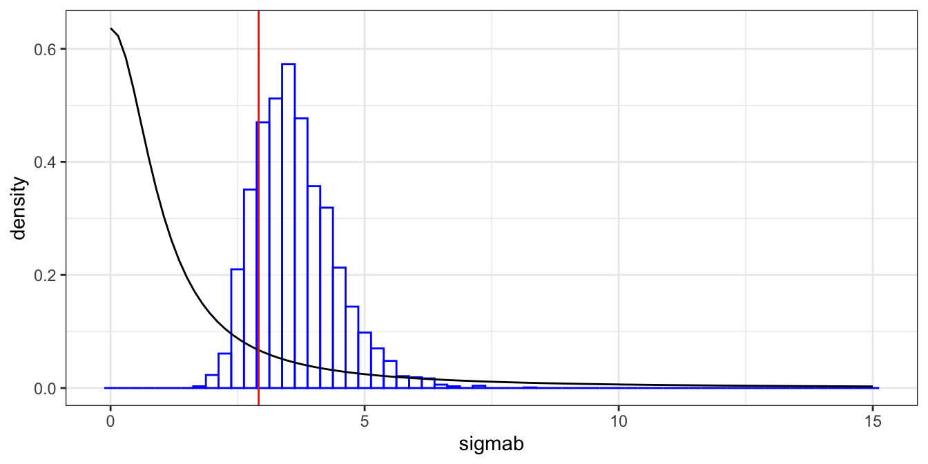
Figure 4.8: Prior and posterior comparison of the subject random effects parameter. The prior density is given (black) along with posterior histogram (blue), and the likelihood-based estimate from lme4 (red).
4.4.4.7 Examining the new subject prediction
Recall that we included a command in our Stan program to sample from the posterior predictive distribution of a new subject who has the same covariate values as subject 1. Note that we are therefore assuming that this individual has the same age, height, weight, etc. as ‘subject 1’, but is not a new observation on that particular subject, but merely a different person with those covariate measurements. We can extract the results of these two variables to obtain a predictive credible interval. Remember that \(\tilde{b}\) is the posterior predicted random effect of the new subject, and \(\tilde{Y}\) is the posterior predicted balance outcome of that subject.
## Inference for Stan model: c808de51faf75c5c13f75aad1c4debdc.
## 4 chains, each with iter=2000; warmup=1000; thin=1;
## post-warmup draws per chain=1000, total post-warmup draws=4000.
##
##         mean se_mean   sd  2.5%   25%   50% 75% 97.5% n_eff Rhat
## bTilde -0.04    0.06 3.79 -7.44 -2.48 -0.05 2.3  7.65  3693    1
## yTilde  0.86    0.01 0.35  0.00  1.00  1.00 1.0  1.00  3667    1
##
## Samples were drawn using NUTS(diag_e) at Sun Mar 20 17:05:22 2022.
## For each parameter, n_eff is a crude measure of effective sample size,
## and Rhat is the potential scale reduction factor on split chains (at
## convergence, Rhat=1).
4.4.5 Comparing Stan and lme4
Let’s compare the results that are obtained from fitting this random effect GLM using a likelihood-based approach (lme4) and a Bayesian approach (rstan). The estimated mean and standard deviation for the fixed effects parameters are given in Table 4.7. We also show these results in Figure 4.9. In this figure, the Bayesian approach from rstan is displayed as posterior credible intervals using the samples from the posterior, whereas the likelihood approach from lme4 is displayed as confidence intervals obtained by applying a normal approximation (i.e. \(2\times s.e.\)).
| Stan mean | Stan sd | lme4 mean | lme4 sd | |
|---|---|---|---|---|
| (Intercept) | -13.000 | 2.340 | -11.2000 | 1.870 |
| Surfacenorm | 8.380 | 1.300 | 7.3300 | 1.070 |
| Visiondome | 0.752 | 0.550 | 0.6780 | 0.530 |
| Visionopen | 7.080 | 1.240 | 6.1400 | 0.993 |
| Sexmale | 2.430 | 2.080 | 1.8900 | 1.650 |
| Age | 0.118 | 2.120 | 0.0502 | 1.630 |
| Weight | -0.619 | 3.760 | -0.0591 | 3.040 |
| Dummy | 0.242 | 0.247 | 0.2400 | 0.231 |
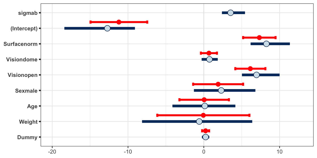
Figure 4.9: Estimates of the parameters in the balance model. The blue circles/bars give the posterior meadian/(0.025,0.975) credible interval from the Bayesian approach, and the red circles/bars give the estimate/(0.025,0.975) approximate confidence interval. Note that lme4 does not report a standard error for random effects parameters.
Additionally, we can explore the subject-specific random effects, including the predictive distribution. Figure 4.10 shows the estimates of the random effects for each of the 40 subjects in the experiment. It also shows the posterior predictive interval for the subject-specific effect of a new, unknown individual. The Bayesian results are shown in blue. For this new individual, we compare with \(\pm 2 \hat{\sigma}_b\), where \(\hat{\sigma}_b\) is the estimate obtained via lme4 (red).
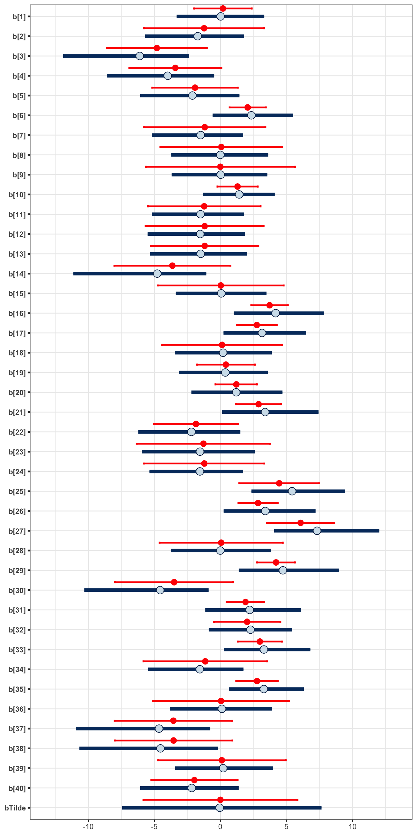
Figure 4.10: Comparison of the subject-specific random effects. The (0.025,0.975) posterior credible intervals of each subject’s effect obtained via a Bayesian approach is shown in blue, and the approximate confidence interval obtained via a likelihood approach is shown in red. In additon to the estimates of the 40 subjects from the experiment, we also include the prediction for a new unknown individual, using bTilde. In blue we show the posterior predictive median (point) and (0.025,0.975) credible predictive interval obtained via the Bayesian approach. In red we show the interval given by plus and minus 2 times the estimate of the random effect deviation.
4.4.6 ‘Easy’ Bayesian approach with brms
We have implemented a Bayesian approach to regression analysis using Stan, and this took a fair amount of set-up, creating the .stan file with the appropriate design matrix construction. The flexibility of creating the .stan file ourselves is that we can define our model however we like, along with the priors and any generated quantities, such as the predictive distribution we sampled from in our example. However, if we do not need to include these flexible choices, there is a rather quick way we can implement this model, using the package brms, that retains the same syntax that we are familiar with from lm and lme4.
glmBrm <- brm(Stable ~ Surface + Vision +
                Sex +
                Age + Weight + Dummy +
                (1 | Subject),
              family = bernoulli,
              data = balance)
We can summarise and compare the output here with what we obtained ourselves in Stan:
summary(glmBrm)## Family: bernoulli
## Links: mu = logit
## Formula: Stable ~ Surface + Vision + Sex + Age + Weight + Dummy + (1 | Subject)
## Data: balance (Number of observations: 480)
## Draws: 4 chains, each with iter = 2000; warmup = 1000; thin = 1;
## total post-warmup draws = 4000
##
## Group-Level Effects:
## ~Subject (Number of levels: 40)
## Estimate Est.Error l-95% CI u-95% CI Rhat Bulk_ESS Tail_ESS
## sd(Intercept) 3.49 0.71 2.30 5.06 1.00 1130 1636
##
## Population-Level Effects:
## Estimate Est.Error l-95% CI u-95% CI Rhat Bulk_ESS Tail_ESS
## Intercept -12.11 2.08 -16.62 -8.48 1.00 1484 1744
## Surfacenorm 8.01 1.18 5.96 10.55 1.00 1755 2021
## Visiondome 0.72 0.56 -0.36 1.84 1.00 4799 2777
## Visionopen 6.76 1.12 4.87 9.26 1.00 1705 1963
## Sexmale 2.03 2.00 -1.77 6.18 1.00 1371 1515
## Age -0.01 1.98 -4.11 3.82 1.00 1566 2195
## Weight -0.03 3.64 -7.06 7.35 1.00 1374 2031
## Dummy 0.24 0.24 -0.22 0.71 1.00 6063 3250
##
## Draws were sampled using sampling(NUTS). For each parameter, Bulk_ESS
## and Tail_ESS are effective sample size measures, and Rhat is the potential
## scale reduction factor on split chains (at convergence, Rhat = 1).As you can see, this approach retains interpretable variable labelling without us needing to, which is a bonus! Comparable results to our analysis in Stan can be seen by the trace plot in Figure 4.11 and the caterpillar plot in Figure 4.12. As we can see, these results are very similar to the Stan implementation. Note that both are stochastic processes so we cannot expect identical results. However, there is an implementation difference here because we used a specified prior in our custom Stan implementation.
## Warning: 'parnames' is deprecated. Please use 'variables' instead.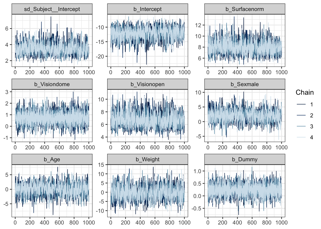
Figure 4.11: Trace plots of the sampled parameters for the balance experiment, fitting a random effects GLM in Stan using the package brms.
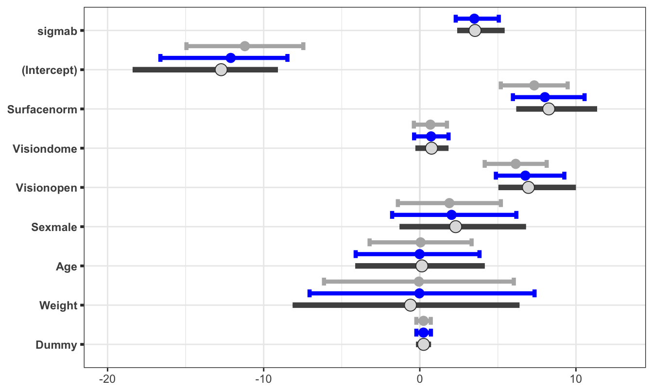
Figure 4.12: Estimates of the parameters in the balance model. The dark grey is the credible interval from the Bayesian approach in Stan, the light grey is the approximate confidence interval from lme4. The new edition here is the blue credible intervals from the Bayesian approach with brms.
4.4.7 What have we found?
The main aim of this example was to explore a sensible process for implementing a regression model using Stan for a non-simplified, real data example. However, it’s useful to summarise our analysis findings nonetheless.
We’ve found that there is significant evidence to suggest that there is a difference in balance for the two surfaces explored, and also between restricted and unrestricted vision. There’s evidence to suggest that there is a small difference between the two ways of restricting vision. There is also evidence to suggest a small difference in balance between the genders, but that other covariates are unlikely to provide useful predictive information. Somewhat comfortingly, we’ve shown (with little uncertainty!) that the dummy variable is uninformative for explaining balance. Finally, we’ve seen evidence of a variation between individuals.
Note that we have not investigated model fit or validity of assumptions here, though this is an important aspect of model fitting analysis.