Chapter 6 Bootstrapping
\(\def \mb{\mathbb}\) \(\def \E{\mb{E}}\) \(\def \P{\mb{P}}\) \(\DeclareMathOperator{\var}{Var}\) \(\DeclareMathOperator{\cov}{Cov}\)
| Aims of this chapter |
|---|
| 1. Introduce bootstrapping: a Monte Carlo method for obtaining standard errors and confidence intervals, and performing hypothesis tests. |
| 2. Understand sampling from the empirical distribution function, or equivalently, resampling observations with replacement, as the key step in the bootstrapping method. |
| 3. Explain the difference between nonparametric and parametric bootstrapping, and show how the latter can be used for hypothesis testing. |
6.1 Bootstrap estimates of standard errors
We will first consider the problem of obtaining standard errors and confidence intervals for parameter estimates.
Suppose we want to estimate a parameter \(\theta\) in some statistical model given a sample of data \(\mathbf{x}=\{x_1,\ldots,x_n\}\). We will use an estimate \[ \hat{\theta}(\mathbf{x}), \] where \(\hat{\theta}(.)\) is some function of the data \(\mathbf{x}\). The standard error of the estimator, denoted by \(s.e.(\hat{\theta})\) is defined as \[ s.e.(\hat{\theta})=\sqrt{Var\{\hat{\theta}(\mathbf{X})\}} \] for a random sample of data \(\mathbf{X}=\{X_1,\ldots,X_n\}\). In other words, before we get the data, we think of \(\hat{\theta}(\mathbf{X})\) as a random variable, and the standard error is the standard deviation of this random variable. For simple problems, we can derive formulae for standard errors.
For example, if we have \[X_1,\ldots,X_n \stackrel{i.i.d}{\sim}N(\theta, \sigma^2),\] and our estimator for \(\theta\) is \(\hat{\theta}(\mathbf{X}) =\bar{X}\), then we can show that \[ s.e.(\hat{\theta}) = \frac{\sigma}{\sqrt{n}}. \] What can we do when we have more complicated models, and we can’t derive formulae such as that above?
Suppose we knew the distribution \(F\) of the data. We could then use a Monte Carlo procedure to estimate a standard error:
- Sample \(N\) independent data sets \(\mathbf{x}^*_1,\ldots,\mathbf{x}^*_N \sim F(\cdot)\), each of size \(n\);
- For each data set \(i\), calculate the corresponding estimate \(\hat{\theta}(\mathbf{x}_i^*)\) of the parameter \(\theta\);
- Estimate the standard error \(s.e.(\hat{\theta})\) by \[ \widehat{s.e.}(\hat{\theta})=\left[\frac{1}{N-1}\sum_{i=1}^N\left\{\hat{\theta}(\mathbf{x}^*_i)-\bar{\hat{\theta}}\right\}^2\right]^{0.5}, \] with \(\bar{\hat{\theta}}=\sum_{i=1}^N \hat{\theta}(\mathbf{x}^*_i)/N\).
This is the bootstrap estimate of the standard error. As long as we can sample datasets in step (1), and then actually calculate a parameter estimate given a data set, it doesn’t matter how complicated the model is. This makes the bootstrapping method widely applicable.
We don’t actually know what \(F\) is (if we did, we would already know all the corresponding parameters), but if we could estimate it, we could do an approximation of the Monte Carlo procedure above, where we instead sample random data sets from our estimate of \(F\). This may seem like a somewhat circular argument: normally it’s the parameter estimates that give us our estimate of the distribution \(F\), but in bootstrapping, we can estimate \(F\) without reference to any particular model; we can estimate \(F\) without having to first estimate any parameters.
6.2 Estimating a distribution using the empirical cumulative distribution function
In (nonparametric) bootstrapping we estimate the distribution \(F\) given observations \(\{x_1,\ldots,x_n\}\) by the empirical cumulative distribution function (ECDF). We denote the ECDF by \(F_n\) and define it as \[ F_n(x) := \frac{1}{n}\sum_{i=1}^n I(x_i \le x), \] where \(I(\cdot)\) is the indicator function.
We illustrate this for \(X_1,\ldots,X_5 \sim N(0, 1)\). Let our observations be \[(x_1,\ldots,x_5) = (-0.897, 0.185, 1.59, -1.13, -0.0803),\] then the ECDF is given by that in Figure 6.1 along with the true distribution function. We can see that this is not a particularly good estimate of the true cumulative distribution function, and so for small sample sizes, we may not expect bootstrapping to work well.
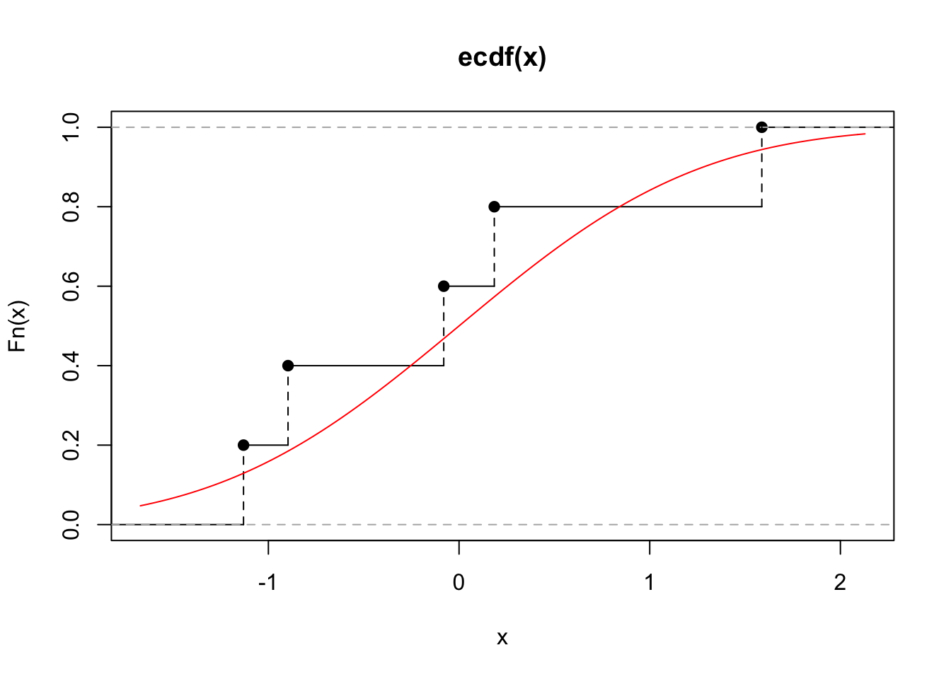
Figure 6.1: The ECDF for five observations drawn independently from a standard normal (black). The true distribution function for the standard normal is shown in red.
However, the estimate will be better for larger sample sizes, e.g. we repeat this process for observations \(x_1,\ldots,x_{50}\) of the i.i.d. random variables \(X_i\sim N(0,1)\), for \(i=1,\ldots,50\) and show this in Figure 6.2.
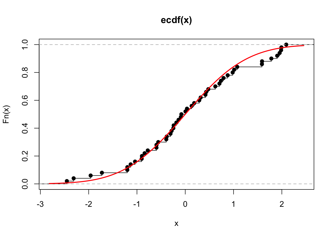
Figure 6.2: The ECDF for 50 observations drawn independently from a standard normal (black). The true distribution function for the standard normal is shown in red.
6.2.1 Sampling from an ECDF
To produce a bootstrap sample of data, we need to generate a sample of size \(n\) (the same size as the original data set) from the ECDF. Sampling from an ECDF is equivalent to sampling randomly from \(\{x_1,\ldots,x_n \}\) with replacement (i.e. where each observation is equally likely to be chosen each time). We therefore don’t actually need to explicitly specify the ECDF! We will demonstrate this shortly, but there are two ways in which we can see that this is valid.
Firstly, if a random variable \(X\) has probability distribution specified by the empirical distribution function for the sample \(\{x_1,\ldots,x_n\}\), then for \(i=1,\ldots,n\) we have \[\begin{align} P(X = x) &= P(X \le x) - P(X < x) \\ &= \frac{1}{n} \sum_{i=1}^n I(x_i \le x) - \frac{1}{n} \sum_{i=1}^n I(x_i < x) \\ & = \frac{1}{n}\sum_{i=1}^n \left(I(x_i \le x) - I(x_i < x)\right) \\ &= \begin{cases} \frac{1}{n} & \text{for } x \in \{x_1,\ldots,x_n\};\\ 0 & \text{otherwise}. \end{cases} \end{align}\] as \(I(x_i \le x) - I(x_i < x) = 1\) if \(x= x_i\) and 0 otherwise.
Secondly, the process can be understood via the inversion method of sampling. Let \(X\) be any random variable with distribution function (CDF) \(F_X(x)\). If we transform \(X\) using its own CDF, i.e. if we define a new random variable \(Y\) as \(Y=F_X(X)\), then it can be shown that \(Y\sim U[0, 1]\). Hence if we can sample \(Y\) from the \(U[0, 1]\) distribution, we can obtain a random draw from the distribution of \(X\) by setting \(X=F_X^{-1}(Y)\).
Now, if \(F_X(x)\) is an ECDF, the function consists of \(n\) ‘steps’ of height all equal \(1/n\), and so when we apply the inversion of a uniform random variable, any point in \(\{x_1,\ldots,x_n\}\) has the same probability of being selected. We see this process in Figure 6.3, where we show the ECDF of five standard uniform samples. If we draw the value \(u\) from a uniform distribution, we apply the inverse function \(F_X^{-1}(u)=x_3\) and so we set \(x_3\) as our random draw.
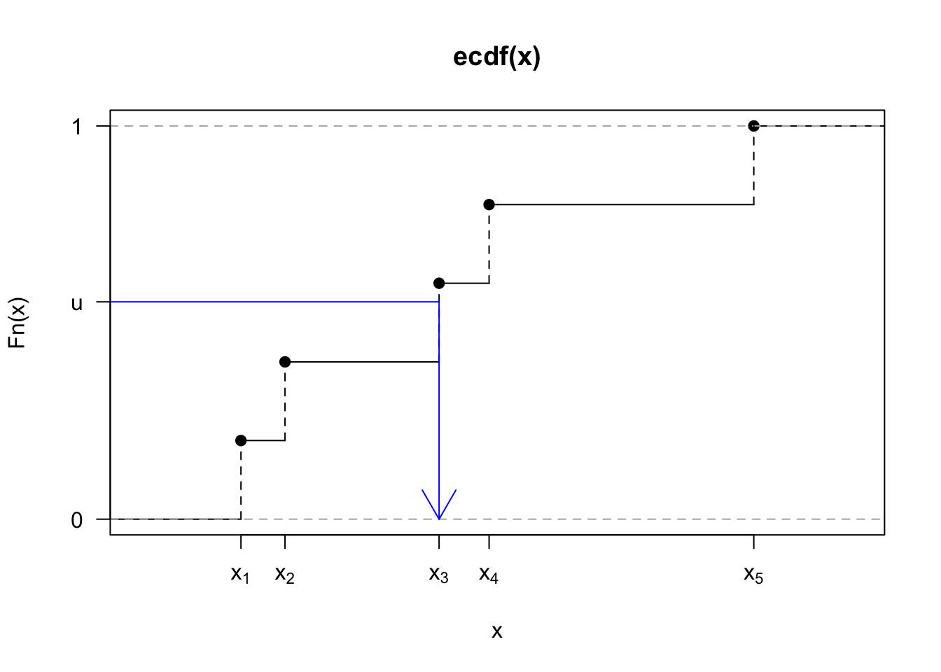
Figure 6.3: The ECDF for five observations drawn independently from a standard normal (black). We sample a value \(u\) from a uniform distribution and apply an inverse transformation \(F_X^{-1}(u)\) to yield the corresponding value of \(x\), which here is given by \(x_3\).
To give an indication that the process of sampling with replacement does indeed work, we illustrate this in Figure 6.4. We sample with replacement from a sample of standard normals 1000 times to obtain the histogram shown in the figure. We can see it is a fair approximation to the true density of the standard normal, which is shown in red.
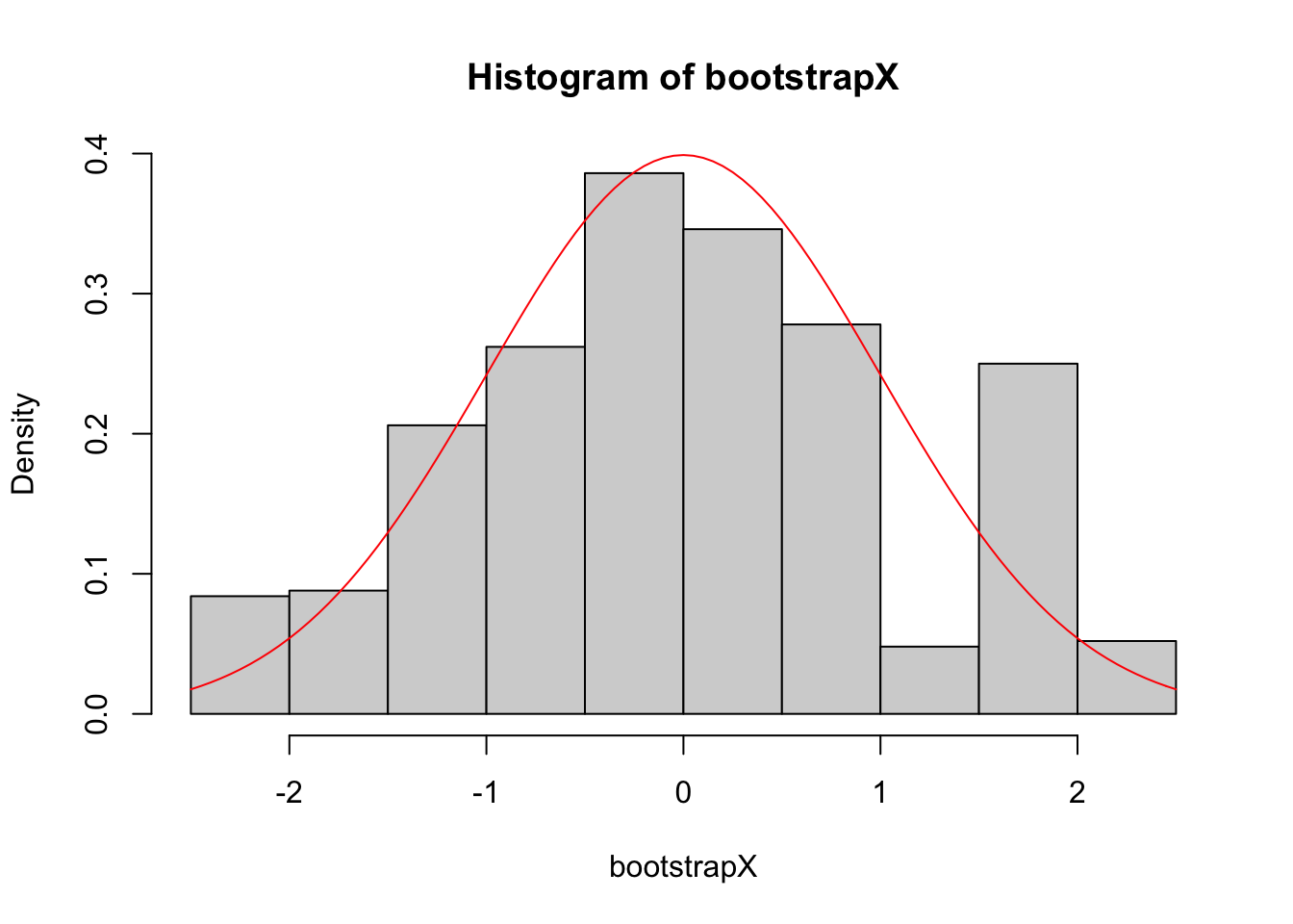
Figure 6.4: Given a sample of 50 independent draws from a standard normal, we sample with replacement 1000 times. This sample is represented by the histogram, and the true density function of the standard normal is shown in red.
6.3 Notation summary
We need to be careful with notation here, as there are various different types of random variables and samples to keep track of. In particular, watch for the ‘big \(X\) random, little \(x\) observed’ distinction, and the use of the \(*\) superscript to indicate the use of bootstrapping. To summarise, we have:
- \(\theta\): a parameter in a model we wish to estimate;
- \(\mathbf{X}=\{X_1,\ldots,X_n\}\): independent and identically distributed random variables, with a probability distribution dependent on \(\theta\);
- \(\mathbf{x}=\{x_1,\ldots,x_n\}\): our observed sample of data;
- \(\mathbf{X^*}=\{X_1^*,\ldots,X_n^*\}\): \(n\) ‘bootstrapped’ random variables, defined by resampling from \(\{x_1,\ldots,x_n\}\) independently and with replacement;
- \(\mathbf{x^*}=\{x_1^*,\ldots,x_n^*\}\): an observed bootstrapped sample
- \(\hat{\theta}(.)\): a function of the data used to estimate \(\theta\);
- \(\hat{\theta}(\mathbf{X})\): an estimator. A random variable, defined as a transformation of the random variables \(\mathbf{X}=\{X_1,\ldots,X_n\}\);
- \(\hat{\theta}(\mathbf{x})\): the estimate we have obtained given the observed data; and
- \(\hat{\theta}(\mathbf{x}^*)\): a bootstrapped estimate of \(\theta\) obtained from a bootstrapped sample of data.
6.4 Example: Bootstrap standard errors of a sample mean and sample variance
We’ll first try bootstrapping in a simple example where we actually know what the true standard errors are, so we can check the method works. We’ll consider normally distributed data \[X_1,\ldots,X_{30}\stackrel{i.i.d}{\sim}N(\mu,\sigma^2).\]
We can use the sample mean \(\bar{X}\) and sample variance \(S^2\) as estimators of \(\mu\) and \(\sigma^2\), and these have standard errors \(\frac{\sigma}{\sqrt{30}}\) and \(\sqrt{\frac{2\sigma^4}{(30 - 1)}}\) respectively. Let’s see if we can recover these known standard errors using a bootstrapping estimate.
We’ll first choose \(\mu=0\) and \(\sigma=1\), and generate a sample of data:
x <- rnorm(30)Now, to obtain a bootstrap sample of data, we just sample the vector x 30 times with replacement, e.g.
bootSample <- sample(x, size = 30, replace = TRUE)and then we would calculate the sample mean and sample variance of bootSample. We repeat this a large number of times to get our sample of estimators:
N <- 10000
bootMeans <- bootVars <- rep(NA, N)
for(i in 1:N){
  bootSample <- sample(x, size = 30, replace = TRUE)
  bootMeans[i] <- mean(bootSample)
  bootVars[i] <- var(bootSample)
}
Now let’s compare the sample standard deviations of our bootstrapped sample of estimators (first value in the pairs calculated below) with the true standard errors that we know from distributional theory (second value in the pairs below). For the sample mean:
c(sd(bootMeans), 1/sqrt(30))## [1] 0.1667101 0.1825742c(sd(bootVars), sqrt(2/29))## [1] 0.2298253 0.2626129In both cases, the bootstrap standard errors are fairly close to the true standard errors.
6.5 Confidence intervals
6.5.1 Confidence intervals using the estimated standard error
If we assume the estimator \(\hat{\theta}\) is normally distributed and unbiased, then once we have the bootstrap estimate of the standard error, \(\widehat{s.e.}(\hat{\theta})\), we can report \[\hat{\theta} \pm 2 \widehat{s.e.}(\hat{\theta}),\] as an approximate 95% confidence interval.
Continuing our example from the previous section, we can compare bootstrap confidence intervals with the exact confidence interval because we can derive that here. We know the distributions of the sample mean \[\bar{X}\sim t_{n-1} \left(\mu,\frac{S}{\sqrt{n}}\right),\] and variance \[S^2\sim \frac{\sigma^2}{n-1}\chi^2_{n-1}.\]
Starting with the mean, the 95% confidence interval for \(\mu\) using the bootstrap approach would be:
c(mean(x) - 2*sd(bootMeans), mean(x) + 2*sd(bootMeans))## [1] -0.2509621 0.4158785and the exact interval would be calculated as \(\bar{x}\pm t_{19;0.025}\sqrt(s^2/20)\):
mean(x) + c(-1,1) * qt(0.975,29) * sd(x) / sqrt(30)## [1] -0.2626142 0.4275306Actually, we can get this interval a little easier in R by fitting a linear model with an intercept only:
confint(lm(x~1))## 2.5 % 97.5 %
## (Intercept) -0.2626142 0.4275306Similarly, for the variance parameter, the 95% confidence interval for \(\sigma^2\) using the bootstrapping approach would be
c(var(x) - 2*sd(bootVars), var(x) + 2*sd(bootVars))## [1] 0.3943486 1.3136500which we can compare with the exact confidence interval \((29s^2/\chi^2_{29;0.025}, \, 29s^2/\chi^2_{29;0.975})\):
(29)*var(x) / qchisq(c(0.975, 0.025), 29)## [1] 0.541661 1.543333The bootstrap interval for the mean is fairly close to the exact interval. The bootstrap interval for the variance is slightly off (though in the right ballpark); we might expect this, as we know that the sample variance \(S^2\) isn’t normally distributed.
6.5.2 Confidence intervals using percentiles
If we think the distribution of the estimator deviates substantially from a normal distribution, we could derive an interval based on percentiles instead. Suppose we could find \(l\) and \(u\) such that
\[\P(\hat{\theta} > \theta + u) = \P(\hat{\theta} < \theta - l) = 0.025,\] then we have \[\P(\hat{\theta} - u<\theta < \hat{\theta} +l)= 0.95.\]
A 95% confidence interval for \(\theta\) would be \[(\hat{\theta} - u,\quad \hat{\theta} +l).\]
We can estimate \(l\) and \(u\) from our bootstrap sample: we estimate these as the 2.5th and 97.5th percentiles from our sample of \(\hat{\theta}(\mathbf{x}^*_i) - \hat{\theta}(\mathbf{x})\) (for \(i=1,\ldots,n\)).
The assumptions here are that:
- The distribution of \(\hat{\theta}(\mathbf{X}) - \theta\) would be the same for any value of \(\theta\), including \(\theta = \hat{\theta}(\mathbf{x})\); and
- The distribution of a randomly generated estimator \(\hat{\theta}(\mathbf{X}^*)\) obtained via bootstrapping is (approximately) the same as the distribution of \(\hat{\theta}(\mathbf{X})\).
In our example, we obtain the confidence interval for \(\sigma^2\) using
var(x) - quantile(bootVars - var(x), c(0.975, 0.025))## 97.5% 2.5%
## 0.4068962 1.2967503In this case, this is not noticeably different from the standard error-based interval. If we plot a histogram of bootstrap estimates, as in Figure 6.5 although the distribution is skewed, the 2.5th and 97.5th percentiles are similar distances from \(\hat{\theta}(\mathbf{x})\).
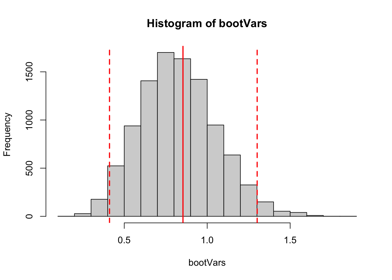
Figure 6.5: A histogram of bootstrapped estimates of the variance. The red solid line shows the sample variance of the observed data, and the dashed lines indicate 2.5th and 97.5th percentiles from the bootstrapped sample of estimates. Although the distribution of bootstrapped estimates is skewed, these percentiles are roughly the same distance from the sample variance.
6.6 Properties of samples from the empirical CDF
6.6.1 Expectation and variance
Following on from the discussion above, it is helpful to understand a little more about what the implications are when we sample from an ECDF. Denote the sample by \(x_1,\ldots,x_n\), and let \(X\) be a random variable sampled from the corresponding ECDF. Then we have \[\begin{align} E(X) &= \sum_{i=1}^n x_i \P(X = x_i) \\ &= \sum_{i=1}^n x_i \frac{1}{n} \\ &= \bar{x}, \end{align}\] and similarly \[E(X^2) = \sum_{i=1}^n x_i^2\frac{1}{n},\] so that \[\var(X) = \frac{n-1}{n}s^2,\] where \(s^2\) is the sample variance.
Hence for a bootstrapped sample mean, we would have \[\var(\bar{X^*}) = \frac{n-1}{n^2}s^2\simeq \frac{s^2}{n}.\] So, for a large enough \(N\), the bootstrap estimate of the standard error of a sample mean would just be (approximately) the usual estimate \(s^2/n\). Therefore, bootstrapping doesn’t add anything to the story here! But, again, the motivation for bootstrapping comes from problems where we could not easily derive standard errors directly rather than the problem of estimating \(\bar{X}\).
6.6.2 Sample percentiles
Suppose we wanted to estimate the standard error of a sample percentile, e.g., the 95th percentile. For a small \(n\), we wouldn’t expect the ECDF to approximate the tails of a distribution particularly well.
Consider, for example, \(n=21\), and denote the ordered sample by \(x_{(1)},\ldots,x_{(21)}\), so that the sample estimate of the 95th percentile (obtained via default algorithm in the quantile() function in R) would be \(x_{(20)}\). In any bootstrap sample, we would frequently obtain \(x_{(20)}\) as the bootstrapped 95th percentile, and we couldn’t get a value larger than \(x_{(21)}\). Therefore, we would likely underestimate the standard error of the sampled 95th percentile (regardless of how many bootstrap samples we take).
We illustrate this as follows. Suppose we have \[X_1,\ldots,X_{21}\stackrel{i.i.d}{\sim}N(\mu, \sigma^2),\] and given the observations \(x_1,\ldots,x_{21}\), we want to give an estimated standard error for the sample 95th percentile. We’ll estimate this with bootstrapping, and in parallel, we’ll also use Monte Carlo to estimate the standard error, using multiple samples of size 21 from the correct distribution.
Here is our approach to estimate the 95th percentile using Bootstrapping and Monte Carlo:
set.seed(1)
x <- sort(rnorm(21)) # obs
N <- 10000 # number of bootstrap samples
boot95th <- sampled95th <- rep(NA, N)

for(i in 1:N){

  # make a bootstrap sample of observations
  bootSample <- sample(x, 21, replace = TRUE)
  # calculate the bootstrap estimator
  boot95th[i] <- quantile(bootSample, 0.95)

  # sample from underlying distribution
  z <- rnorm(21)
  # calculate the estimator
  sampled95th[i] <- quantile(z, 0.95)
}
We compare the standard errors of our samples of the estimator:
sd(boot95th)## [1] 0.2629693sd(sampled95th)## [1] 0.3981949We see that the bootstrap estimate of the standard error is noticeably smaller than that obtained via Monte Carlo. We can see the problem clearer when we compare histograms of the percentile estimates, as in Figure 6.6. We see that there is a limited range of values that can be obtained for the percentile estimate in bootstrapping, and that the standard error of this estimate is an under-approximation.
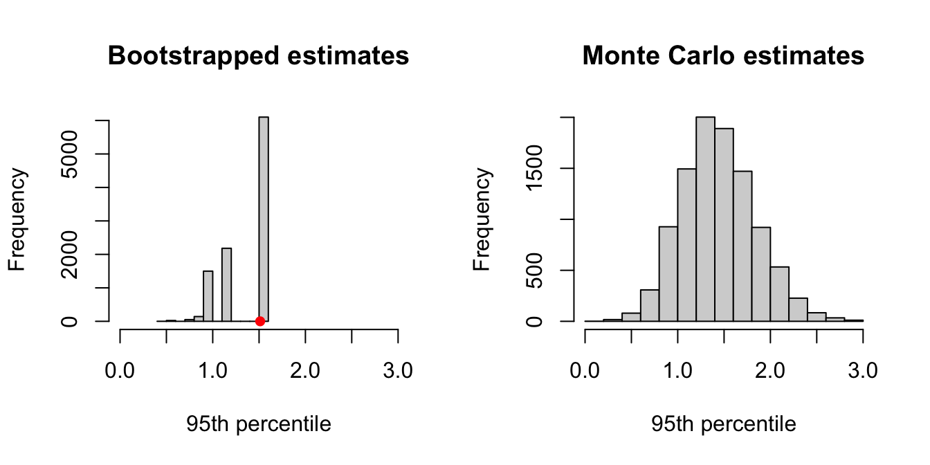
Figure 6.6: Comparison of bootstrapping and Monte Carlo when estimating the 95th percentile from a set of 21 observations. Both methods implemented 10000 samples.
6.6.3 Sources of error and sample sizes in bootstrapping
There are two sources of error to consider in bootstrapping, related to two sample sizes:
- Error in approximating the distribution of the data by the empirical distribution function, based on \(n\) observations;
- Monte Carlo error in estimating a standard error (or some other summary), based on a random sample of \(N\) bootstrapped data sets.
We can usually make \(N\) as large as we want, so that any Monte Carlo error will be negligibly small, but this won’t have any effect on the first source of error. So if the original sample size \(n\) is too small, then by making \(N\) large, we may simply be obtaining a precise Monte Carlo estimate of a poor approximation.
6.7 Example: Measuring observer agreement
So far, we’ve only illustrated bootstrapping in an example where we don’t really need to use it; standard errors and confidence intervals could be obtained analytically. We’ll now consider an example where it’s not so straightforward to derive a confidence interval (although an asymptotic approximation is available).
6.7.1 The data
We consider the diagnoses data set in the irr package (Gamer, Lemon, and <puspendra.pusp22@gmail.com> 2019). We have psychiatric diagnoses for 30 patients. Each patient has been diagnosed separately by 6 different ‘raters’, and the interest is in the extent to which the raters agree with each other. There are five possible diagnoses: depression; personality disorder, schizophrenia, neurosis, “other”.
We’ll just consider diagnoses made by the first two raters, an extract of this data is shown in Table 6.1. These two raters agreed on five out of their first six diagnoses.
| rater1 | rater2 |
|---|---|
| 4. Neurosis | 4. Neurosis |
| 2. Personality Disorder | 2. Personality Disorder |
| 2. Personality Disorder | 3. Schizophrenia |
| 5. Other | 5. Other |
| 2. Personality Disorder | 2. Personality Disorder |
| 1. Depression | 1. Depression |
6.7.2 The kappa statistic
One way to measure agreement between raters is to use Cohen’s kappa statistic, defined as \[\kappa := \frac{p_o - p_e}{1 - p_e},\] where \(p_o\) is the observed proportion of times two raters agreed, and \(p_e\) is the estimated probability the raters would agree purely by chance (i.e. the diagnosis given by rater 1 is probabilistically independent of the diagnosis given by rater 2). In our example, we would obtain \(p_e\) as \[p_e = \sum_{j=1}^5 p_{1,j}p_{2,j},\] where \(p_{i,j}\) is the observed proportion of times rater \(i\) gave diagnosis \(j\).
A kappa of 1 would correspond to perfect agreement, and a kappa of 0 would correspond to agreement no better than chance. Note that kappa can be negative if the agreement is worse than that expected by chance.
In R, we can compute kappa using the function irr::kappa2():
##  Cohen's Kappa for 2 Raters (Weights: unweighted)
##
##  Subjects = 30
##    Raters = 2
##     Kappa = 0.651
##
##         z = 7
##   p-value = 2.63e-12
We obtained \(\kappa = 0.651\) in this example: interpreting the actual value can be hard, but comparing relative values may be helpful for comparing how well different pairs of raters agree with each other. And since we calculated kappa using 30 observations only, it may be helpful to obtain a confidence interval, to assess uncertainty in this value.
6.7.3 Bootstrapping bivariate data
For the two raters, denote the data by \[\begin{align} (r_{1, 1}&, r_{2, 1}) \\ &\vdots \\ (r_{1,30}&, r_{2,30}), \end{align}\] where \(r_{i,j}\) is the diagnosis given by rater \(i\) for observation \(j\). To get a bootstrap sample, we resample pairs of diagnoses, with replacement, which we can do by sampling from the indices 1-30 of our data:
indices <- 1:30
(bootIndex <- sample(indices, size = 30, replace = TRUE))
## [1] 25 4 7 1 2 29 23 11 14 18 27 19 1 21 21 10 22 14 10 7 9 15 21 5 9
## [26] 25 14 5 5 2so the first element of our bootstrap sample is \((r_{1,25}, r_{2,25})\), the second element is \((r_{1,4}, r_{2,4})\) and so on. We then recompute kappa for each bootstrap sample. For example:
N <- 1000
bootKappa <- rep(0, N)
for(i in 1:N){
  bootIndex <- sample(indices,
                      size = 30,
                      replace = TRUE)
  bootData <- diag2[bootIndex, ]
  bootKappa[i] <- irr::kappa2(bootData)$value
}
We can now extract sample quantiles from our bootstrapped sample of kappa values, to get our approximate confidence interval:
quantile(bootKappa, probs = c(0.025, 0.975))## 2.5% 97.5%
## 0.4451596 0.8516323Although we have only considered the first two raters here, to give these numbers a little more context, we show the range of observed kappa statistics between rater 1 and each of the other four raters: 0.384, 0.258, 0.188, and 0.0809, so these range from 0.08-0.38. We may therefore conclude that there is evidence of agreement between the first two raters.
6.8 Parametric bootstrapping and hypothesis testing
So far in this chapter we have considered nonparametric bootstrapping.
In parametric bootstrapping, we first fit a parametric distribution to our data, and then sample new data sets from this distribution, rather than the nonparametric approach of resampling our observed data. This can be useful in hypothesis testing problems in which it is difficult to work out the distribution of the test statistic under the null hypothesis; we can use Monte Carlo instead.
We illustrate this with an example in mixed effects modelling.
6.8.1 The Milk data set
Our example will use the Milk data from the nlme package (Pinheiro et al. 2021), an extract of which is given in Table 6.2.
| protein | Time | Cow | Diet |
|---|---|---|---|
| 3.63 | 1 | B01 | barley |
| 3.57 | 2 | B01 | barley |
| 3.47 | 3 | B01 | barley |
| 3.65 | 4 | B01 | barley |
| 3.89 | 5 | B01 | barley |
| 3.73 | 6 | B01 | barley |
This data features the following variables:
proteinis the dependent variable: the protein content of in a sample of cow milk;Cowlabels the cow from which the sample was taken;Timeis the number of weeks since calving for the correspondingCow; andDietis one of three possible diets the cow was on (barley,lupins,barley+lupins).
Multiple samples are taken from each cow, and we might expect correlation between observations taken on the same cow. The plot in Figure 6.7 confirms this.
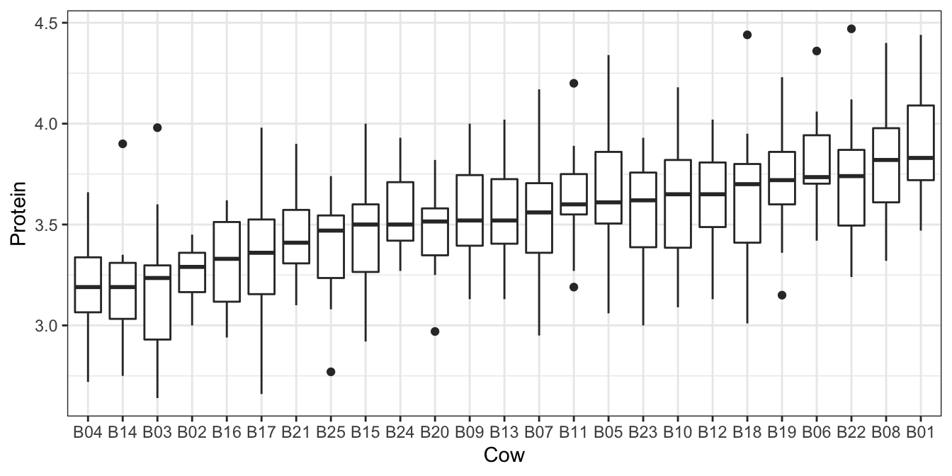
Figure 6.7: Protein content of milk from repeated measures across different cows from the milk dataset.
Each cow is assigned to one diet only, so we could not model the effects of both cow and diet as fixed effects. Assuming the interest is really in the ‘population’ of cows, rather than the cows in this particular data set, it makes sense to model the effects of the cows as random effects.
Plotting protein against time in Figure 6.8, we see a clear drop after week 1. We’ll introduce an indicator variable for whether the sample was taken in week 1, but otherwise not model the effect of time.
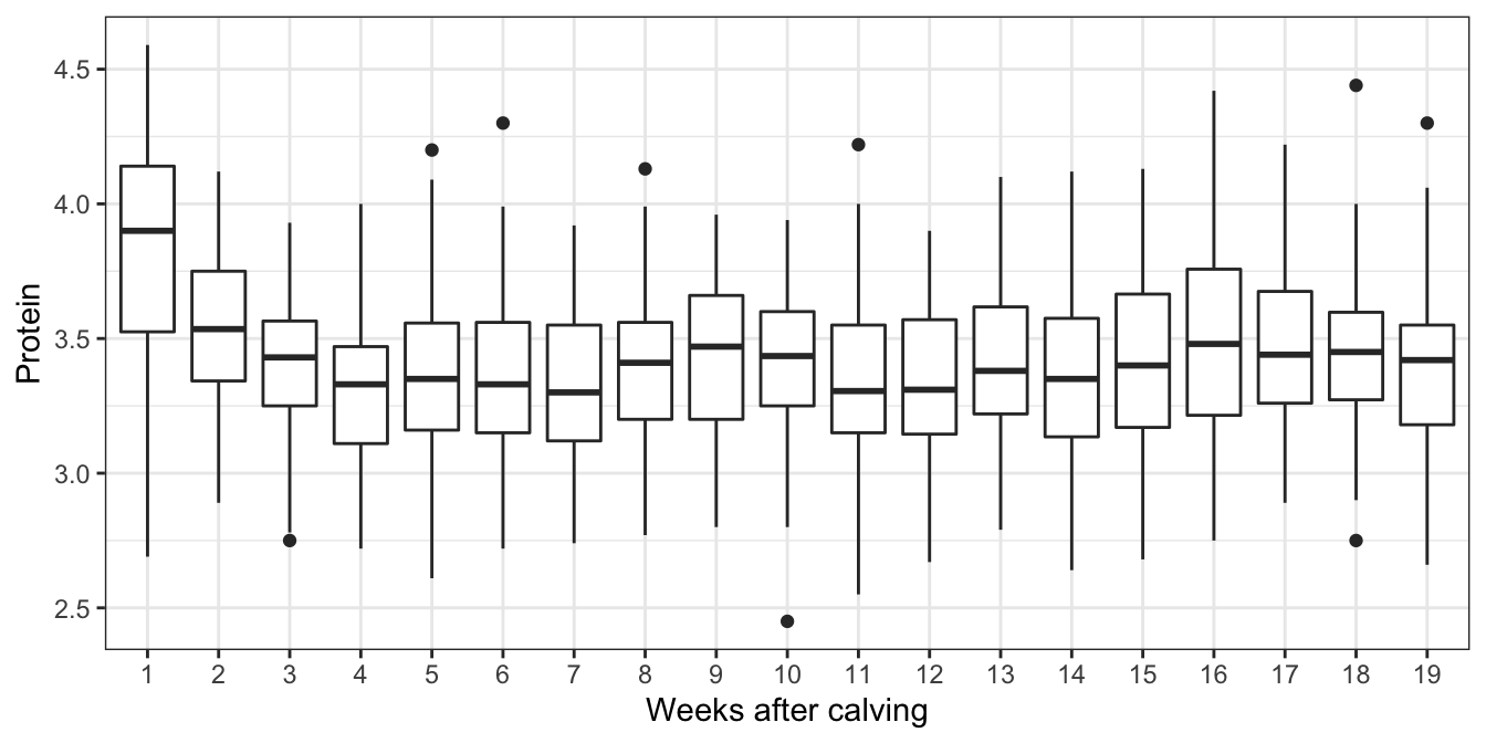
Figure 6.8: Milk yields observed at different weeks after calving. A simple approach to model the effect of time would be to assume yields change after week 1, but are constant, on average thereafter.
We’ll create a new data frame milkDF, with the indicator variable added:
milkDF <- nlme::Milk %>%
  mutate(weekOne = Time == 1)
6.8.2 The model and hypothesis
We consider the model \[ Y_{ijt} = \mu + \tau_i + \beta I(t=1) + b_{ij} + \varepsilon_{ijt}, \] with
- \(Y_{ijt}\): the protein content at time \(t = 1,\ldots,19\), for cow \(j=1,\ldots,n_i\) within group (diet) \(i=1,2,3\);
- \(\mu\): the expected protein content for a cow on diet 1 at time \(t>1\);
- \(\tau_i\): a fixed effect for diet \(i\), with \(\tau_1\) constrained to be 0;
- \(\beta\): the increase in expected protein content at time \(t=1\);
- \(b_{ij}\sim N(0, \sigma^2_b)\), a random effect for each cow;
- \(\varepsilon_{ijt}\sim N(0, \sigma^2)\) a random error term.
We suppose the null hypothesis of interest is \[ H_0: \tau_2=\tau_3=0, \] so that diet has no effect on protein levels. The alternative hypothesis is that at least one \(\tau_i\) is non-zero. One way to do this test would be to use the generalised likelihood ratio test, which we recap in the following section.
6.8.3 The generalized likelihood ratio test
We use the following notation. Suppose observations are independent and the \(i^\text{th}\) observation is drawn from the density (or probability function, if discrete) \(f(y; x, \psi)\) where \(\psi\) is a vector of unknown parameters, and \(x\) is a vector of any corresponding independent variables Then the likelihood and log-likelihood of the observations are \[\begin{align*} L(\mathbf{y};\,\mathbf{x},\, \psi)&= \prod_i f(y_i;\, x_i, \psi),\\ \ell(\mathbf{y};\,\mathbf{x},\, \psi)&:= \log L(\mathbf{y};\,\mathbf{x},\, \psi)= \sum_i \log f(y_i; x_i, \psi), \end{align*}\] respectively.
Now suppose that a simplification is proposed that entails imposing \(r\) restrictions, \(s_i(\psi)=0\) for \(i=1,\ldots, r\), on the elements of \(\psi\), where \(r\) is less than the number of components in \(\psi\). These restrictions must be functionally independent, which is another way of saying all \(r\) of them are needed. In our example, we have two restrictions: \(\tau_2=0\) and \(\tau_3 = 0\). Suppose the maximum likelihood for the restricted situation is \(\widehat{\psi}_s\), which is obtained by maximising \(\ell\) subject to the constraints. When the simpler model is correct, approximately \[ - 2 \left( \ell(\mathbf{y};\,\mathbf{x},\, \widehat{\psi}_s)- \ell(\mathbf{y};\,\mathbf{x},\, \widehat{\psi}) \right) \sim \chi^{2}_{r} \] That is, twice the difference between the maximised value of the log-likelihood from the simpler model and that for the more complex one is approximately \(\chi^{2}_{r}\). On the other hand, if the simpler model is false the difference between these two is expected to be large; hence this theory can be used as the basis of a test, called the generalized likelihood ratio test (GLRT).
To summarise, to conduct a GLRT, we do the following:
- Evaluate the maximised log-likelihood \(\ell(\mathbf{y};\,\mathbf{x},\,\hat{\psi})\).
- Evaluate the maximised log-likelihood \(\ell(\mathbf{y};\,\mathbf{x},\,\hat{\psi}_s)\) with \(\psi\) constrained according to the null hypothesis.
- Evaluate the test statistic \[ L=-2\left(\ell(\mathbf{y};\,\mathbf{x},\,\hat{\psi}_s)-\ell(\mathbf{y};\,\mathbf{x},\,\hat{\psi})\right). \] and compare with the \(\chi^2_r\) distribution, where \(r\) is the number of constraints specified by the null hypothesis. So, if for example we find \(L>\chi^2_{r;0.95}\), we would reject \(H_0\) at the 5% level.
Various standard hypothesis tests can be constructed from the GLRT. In some cases we can derive the exact distribution of \(L\), rather than using the \(\chi^2\) approximation, and in some other cases, the distribution of \(L\) is \(\chi^2_r\) anyway.
However, for mixed effects models, and when testing fixed effects Pinheiro and Bates (2005, Section 2.4.2) say that this test can sometimes be badly anti-conservative, that is, it can produce p-values that are too small. Parametric bootstrapping gives us another way to do the test, without relying on the \(\chi^2_r\) approximation.
6.8.4 The parametric bootstrap test
We need to simulate values of \(L\) under the condition that \(H_0\) is true. One way to do this is to fit the reduced model to the data, then simulate new values of the dependent variables, keeping the independent variables the same, and assuming the parameters are equal to their estimated values. The algorithm is therefore:
- Calculate the GLRT statistic for the observed data. Denote the value of the statistic by \(L_{obs}\).
- Fit the reduced model under \(H_0\) to the data (i.e. leave out the
Dietvariable in our example). - Simulate new values of \(Y_{ijt}\) for \(i=1,2,3\), \(j=1,\ldots,n_i\) and \(t=1,\ldots,19\) from the reduced model. This is our bootstrapped data set, but generated from a parametric model, rather than from an ECDF.
- For the simulated data \(\mathbf{y}^*\), calculate the GLRT statistic \[ L=-2\left(\ell(\mathbf{y}^*;\,\mathbf{x},\,\hat{\psi}_s)-\ell(\mathbf{y}^*;\,\mathbf{x},\,\hat{\psi})\right). \]
- Repeat steps 3-4 \(N\) times, to get a sample of GLRT statistics \(L_1,\ldots,L_N\).
- Estimate the \(p\)-value by \[\frac{1}{N}\sum_{i=1}^N I (L_i\ge L_{obs}).\]
6.8.5 Implementation with R
We first do the standard GLRT in R, using the lme4 package (Bates et al. 2015) to fit the models. One technical detail that we won’t worry too much about here is that we need to use ‘ordinary’ maximum likelihood rather than ‘restricted’ maximum likelihood (REML) for this test, even though the latter is preferred for model fitting.
We fit the full model and extract the maximised log likelihood:
fmFull <- lmer(protein ~ Diet  + weekOne + (1|Cow),
               REML = FALSE,
               data = milkDF)
logLik(fmFull)
## 'log Lik.' -147.7877 (df=6)We then fit our reduced model under \(H_0\), and extract the maximised log likelihood:
fmReduced <- lmer(protein ~ weekOne +(1|Cow),
                  REML = FALSE,
                  data = milkDF)
logLik(fmReduced)
## 'log Lik.' -155.5944 (df=4)We can now compute an observed test statistic, and calculate a \(p\)-value, using the \(\chi^2_r\) distribution, here with \(r=2\).
obsTestStat<- as.numeric(- 2*(logLik(fmReduced)
                              -logLik(fmFull)))
1 - pchisq(obsTestStat, 1)
## [1] 7.770794e-05Here, obsTestStat is step (1) of our approach listed above.
Now we simulate test statistics using parametric bootstrapping; we simulate new data sets from the reduced model (step 3 in the above). We can use the simulate() function to do this:
set.seed(123)
N <- 1000
sampleTestStat<-rep(NA, N)

for(i in 1:N){

  # simulate new data (step 3)
  newY <- unlist(simulate(fmReduced))

  # calculate the test statistic under the simulated data (step 4)
  fmReducedNew<-lmer(newY ~ milkDF$weekOne  +
                       (1|milkDF$Cow),
                     REML = FALSE)
  fmFullNew <- lmer(newY ~ milkDF$Diet + milkDF$weekOne  +
                      (1|milkDF$Cow),
                    REML = FALSE)
  sampleTestStat[i] <- -2*(logLik(fmReducedNew) - logLik(fmFullNew))
}
Now we’ll count the proportion of bootstrapped test statistics greater than or equal to our observed one (step 6):
mean(sampleTestStat >= obsTestStat)## [1] 0We didn’t actually generate any test statistics as large as the observed one, so we’d need to generate more to get an estimated \(p\)-value. But if we compare the distribution of sampled test statistics with the \(\chi^2_2\) distribution, they are fairly similar. This is shown in Figure 6.9.
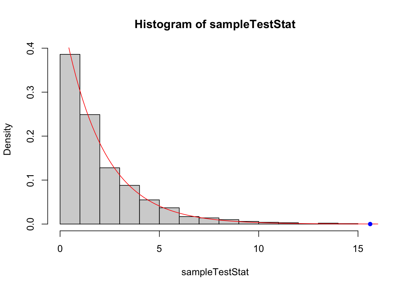
Figure 6.9: Comparing the distribution of the test statistic from bootstrapping (histogram) with the \(\chi^2_2\) approximation used in the generalised likelihood ratio test. The agreement looks fairly good here. The blue dot indicates the observed test statistic.
So the use of bootstrapping hasn’t changed our conclusion here, but has given us a means of checking whether the distribution assumed in the GLRT is appropriate.