Chapter 3 Implementing HMC in Stan
\(\def \mb{\mathbb}\) \(\def \E{\mb{E}}\) \(\def \P{\mb{P}}\) \(\DeclareMathOperator{\var}{Var}\) \(\DeclareMathOperator{\cov}{Cov}\)
| Aims of this chapter |
|---|
| 1. Implement Hamiltonian Monte Carlo using Stan and gain confidence interpreting analyses. |
In this Chapter, we will take a first look at using Stan (implemented via the rstan package (Stan Development Team 2021)) to implement HMC. We will also look at some additional R packages which are useful for working with output from rstan.
This Chapter is only intended to introduce you to using Stan; it will not cover everything you might need to know. Further reading is discussed at the end of this Chapter.
3.1 Getting set up with Stan
In this course we will use RStudio to write, edit and run Stan code. Please ensure that you have an up-to-date version of Rstudio and R itself on your machine.
You can follow the installation steps at the RStan Getting Started page, but we will also summarise these:
- You will need R version 3.4.0 or later (version 4.0.0 or later is strongly recommended)
- You will need RStudio version 1.2.x or later (version 1.4.x or later is strongly recommended. Note that version numbering system has changed! Version numbers now start with the year: anything starting with 2022 is newer than 1.4.x).
- You need to be able to compile C++ code in R. Windows users will need to install RTools. Mac users may be prompted to install/update Xcode. The above page links to the appropriate option for Windows, Mac and Linux users.
- You need to install the
RStanpackage in RStudio.
3.2 rstan options
When you run the command
library(rstan)you will get some text recommending you set two options:
options(mc.cores = parallel::detectCores())
rstan_options(auto_write = TRUE)
We suggest you try both. The first will enable parallel processing on your computer. The second will save your Stan models to a temporary folder on your hard drive, which may save a little time if you find yourself recompiling models in the same session.
3.3 An example model
For our first implementation in Stan, we will introduce a simple model. We have \(n\) random variables \(Y_1,\ldots,Y_n\) that are assumed to be independent and identically distributed with \[\begin{equation} Y_i |\mu, \sigma^2 \sim N(\mu,\sigma^2). \end{equation}\] Prior distributions are specified by \[\begin{align} \mu &\sim N(1.5,0.1^2), \\ \sigma &\sim \Gamma(1,1). \end{align}\] Denoting the observations by \(y_1,\ldots,y_n\), we wish to sample from two distributions:
- the posterior distribution of \(\mu,\sigma^2 | y_1,\ldots,y_n\);
- the predictive distribution of \(Y_{n+1},Y_{n+2}|y_1,\ldots,y_n\).
3.4 Specifying a model in RStudio
In RStudio, we make a stan code block. The code block has an argument output.var, defined as a string: we will use the string "ex1". When we click on the green arrow at the top right of the code chunk, the model will be compiled as a “stanmodel” object called ex1.
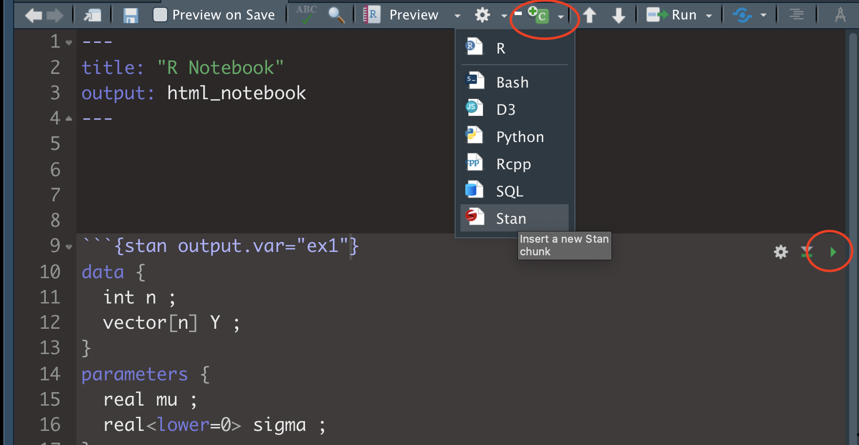
The model code (that goes inside the code block) is as follows. Note that each commands needs to end in a semicolon.
data {
    int n ;
    vector[n] Y ;
}
parameters {
    real mu ;
    real<lower=0> sigma ;
}
model {
    mu ~ normal(1.5, 0.1) ;
    sigma ~ gamma(1, 1) ;
    Y ~ normal(mu, sigma) ;
}
generated quantities {
  vector[2] Ynew ;
  for (i in 1:2)
    Ynew[i] = normal_rng(mu, sigma) ;
}
3.5 Stan code blocks
The code is divided into Stan ‘code blocks’. We’ve used four different types (there are a few others) which we will discuss in turn.
3.5.1 data block
data {
    int n ;
    vector[n] Y ;
}
This is where we declare the data we will pass to Stan for use in our statistical inference. We must declare all our data, and its type.
Here, we have said that the variable \(Y\) is vector, with each element an unbounded continuous variable. For flexibility here, we’ve also included the number of observations \(n\) as an integer variable to let Stan know how large our vector of observations is. If we knew that we had, say 10, observations, we could have defined
vector[10] Y ;directly.Common examples of data types include
real,int,vector, andmatrix.We can also attach modifiers, such as truncated variables asreal<lower=0,upper=1>.
3.5.2 parameters block
parameters {
    real mu ;
    real<lower=0> sigma ;
}
This is where we declare all the parameters of our model that we aim to infer. Here we have the two parameters:
- \(\mu\), which is an unbounded continuous random variable, and
- \(\sigma\), which is a positive continuous random variable.
In addition to the above data types, there are some additional useful parameter data types. This includes simplex, which is a vector of non-negative continuous variables whose sum is 1 and is useful for multinomial parameter sets or other probabilities. Also corr_matrix behaves as expected, and ordered allows the common constraint of \(Z[1]>Z[2]>\ldots>Z[k]\) to be described conveniently.
3.5.3 model block
model {
    mu ~ normal(1.5, 0.1) ;
    sigma ~ gamma(1, 1) ;
    Y ~ normal(mu, sigma) ;
}
This is where we specify our likelihood and priors. This block is essentially telling Stan how to calculate the negative log posterior probability density (up to proportionality) which would be used to calculate the energy.
In the above you will see we have used what is called sampling statements, which are denoted with the \(\sim\) symbol. These describe the sampling distribution of the variables, and is not an instruction to draw a sample from such a distribution.
Though
muis a scalar andYis a vector, we have used the same type of sampling statement:mu ~ normal()andY ~ normal(). Stan will understand the difference and interpret the elements of Y to be i.i.d. with the specified distribution.Stan understands a wide range of standard families of distributions, including all those from your distribution table. Note that these begin with a capital letter only where appropriate (such as
Student-tbut notgamma).
3.5.3.1 Improper priors
We could leave out specification of prior distributions for \(\mu\) and \(\sigma\):
model {
    Y ~ normal(mu, sigma) ;
}
This will assume improper uniform priors (with the constraint that sigma is positive). As you have seen in semester 1, the data will dominate the prior as the sample size increases, so this specification may be convenient in such cases, but robustness to the choice of prior (whether informative or uninformative) should always be investigated.
3.5.4 generated quantities block
generated quantities {
  vector[2] Ynew ;
  for (i in 1:2)
    Ynew[i] = normal_rng(mu, sigma) ;
}
Here we define any quantities that we want Stan to simulate.
We need to declare that
Ynewis avectorwith 2 elements, before we can assign randomly generated values toYnew.We’ve used the function
normal_rng()(rather than the functionnormal()) to generate a normally distributed random variable with meanmuand standard deviationsigma.The
normal_rng()function generates a scalar random variable, so we’ve had to use aforloop to generate i.i.d. variables: the elements of the vectorYnew.
3.6 Running the HMC algorithm
We’ll first make up some data for the example:
exampleY <- rnorm(10, 1.6, 0.2)We then make a list with data specified in the Stan data code block:
exampleData <- list(n = length(exampleY), Y = exampleY)We are going to run a single chain sampler of 10000 iterations, but discard the first half as burn-in. We use the sampling function to carry out HMC sampling, using the definition of our Stan model that we assigned to the name ex1 in the stan code chunk from above, and store this as fit.
sampling_iterations <- 1e4
fit <- sampling(ex1,
                data = exampleData,
                chains = 1,
                iter = sampling_iterations,
                warmup = sampling_iterations/2)
Now we will explore the output samples that Stan has provided from a HMC sampler. There are many ways that we can view results, starting with a simple print-out of a summary, shown below.
fit## Inference for Stan model: 72072a3a3945e2d4332cba14d76c3dd9.
## 1 chains, each with iter=10000; warmup=5000; thin=1;
## post-warmup draws per chain=5000, total post-warmup draws=5000.
##
## mean se_mean sd 2.5% 25% 50% 75% 97.5% n_eff Rhat
## mu 1.62 0.00 0.06 1.50 1.59 1.63 1.66 1.73 2675 1
## sigma 0.20 0.00 0.06 0.12 0.16 0.19 0.23 0.36 2252 1
## Ynew[1] 1.62 0.00 0.22 1.17 1.49 1.63 1.75 2.03 4670 1
## Ynew[2] 1.62 0.00 0.22 1.15 1.50 1.62 1.76 2.05 5063 1
## lp__ 9.03 0.03 1.08 6.12 8.63 9.37 9.81 10.09 1768 1
##
## Samples were drawn using NUTS(diag_e) at Sun Mar 20 17:03:59 2022.
## For each parameter, n_eff is a crude measure of effective sample size,
## and Rhat is the potential scale reduction factor on split chains (at
## convergence, Rhat=1).This includes:
- Information about our implementation, including the number of chains and their length.
- A table of the variables we have sampled (\(\mu\) and \(\sigma\)), and the log probability of the model (
lp):- The posterior mean and standard deviation.
- An estimate of effective sample size for each parameter, which can give us some indication about the autocorrelation in our chain.
- The posterior mean and standard deviation.
- Information about the sampling algorithm, which includes an indication of the efficiency of the sampler.
3.7 Extracting and analysing the samples
We extract the raw samples as follows
chains <- rstan::extract(fit)
names(chains)
## [1] "mu" "sigma" "Ynew" "lp__"Then we can do things such as:
summary(chains$mu)## Min. 1st Qu. Median Mean 3rd Qu. Max.
## 1.382 1.588 1.625 1.622 1.661 1.8043.7.1 R packages for plotting outputs
3.7.1.1 ggmcmc
An excellent package for exploring the output of an MCMC sample is ggmcmc (Fernández-i-Marín 2016), which you can also use for the results of samplers that you have written yourself rather than merely Stan samplers. In the following we highlight some popular plots from this package that can be used to summaries our sampler.
In Figure 3.1, we plot the posterior marginals as separate one-dimensional density estimates, alongside the two-dimensional samples themselves.
# extract the posterior groups in a format that ggmcmc likes
samples <- ggmcmc::ggs(fit)
ggmcmc::ggs_pairs(samples)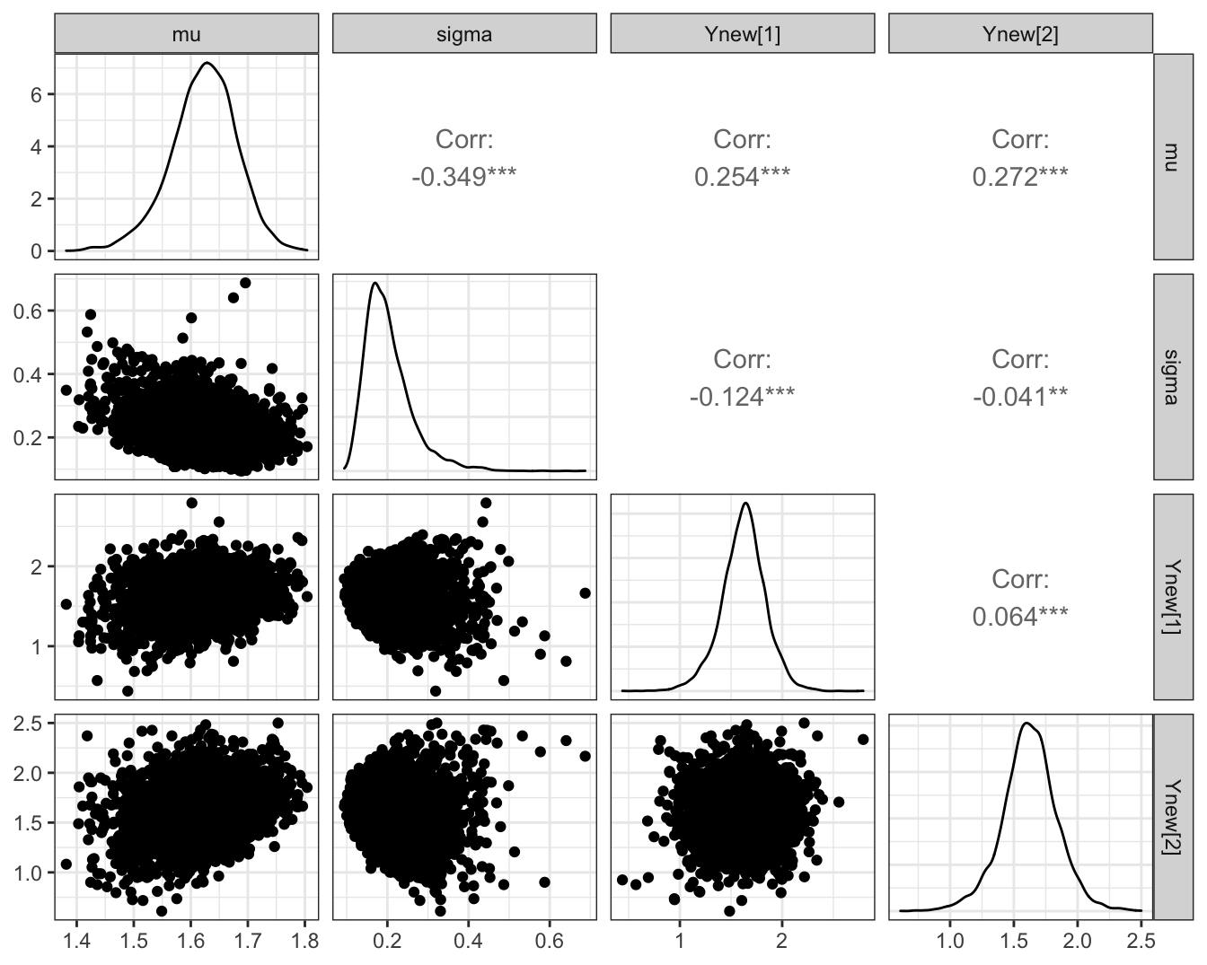
Figure 3.1: Posterior density estimate of the two parameters in the Gaussian example implemented in Stan.
In Figure 3.2, we plot a caterpillar plot, which gives displays credible intervals for each parameter. Compare this with the information table provided in the summary table, above. This is extremely useful for cases with high numbers of estimated parameters (see the random effects regression model later in this course!).
ggmcmc::ggs_caterpillar(samples, thick_ci = c(0.25,0.75))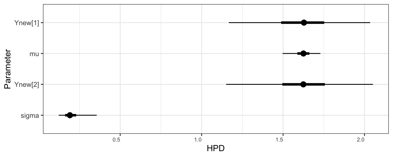
Figure 3.2: Caterpillar plot of the two parameters in the Gaussian example implemented in Stan. The thick bars indicate a posterior quantiles at 0.25 and 0.75, and the thin bards indicate quantiles at 0.025 and 0.975.
Figure 3.3 gives the trace plot of the two parameters, highlighting the autocorrelation in the sampled chain.
ggmcmc::ggs_traceplot(samples)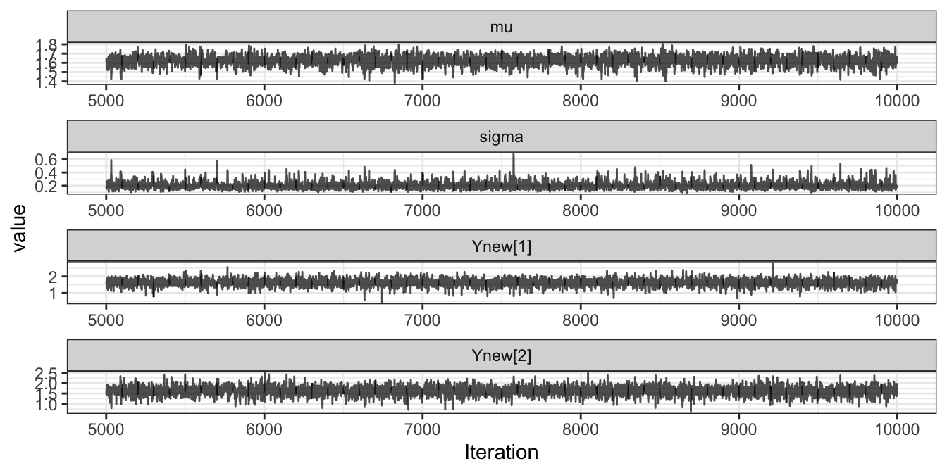
Figure 3.3: Trace plot of the two parameters in the Gaussian example implemented in Stan.
3.7.1.2 bayesplot
The package bayesplot (Gabry and Mahr 2021) interfaces nicely with stan. Trace plots can be produced as follows. Note that vectors are specified within the contains() function.
bayesplot::mcmc_trace(fit,
                      pars = vars(contains("Ynew"),
                                  "mu",
                                  "sigma"))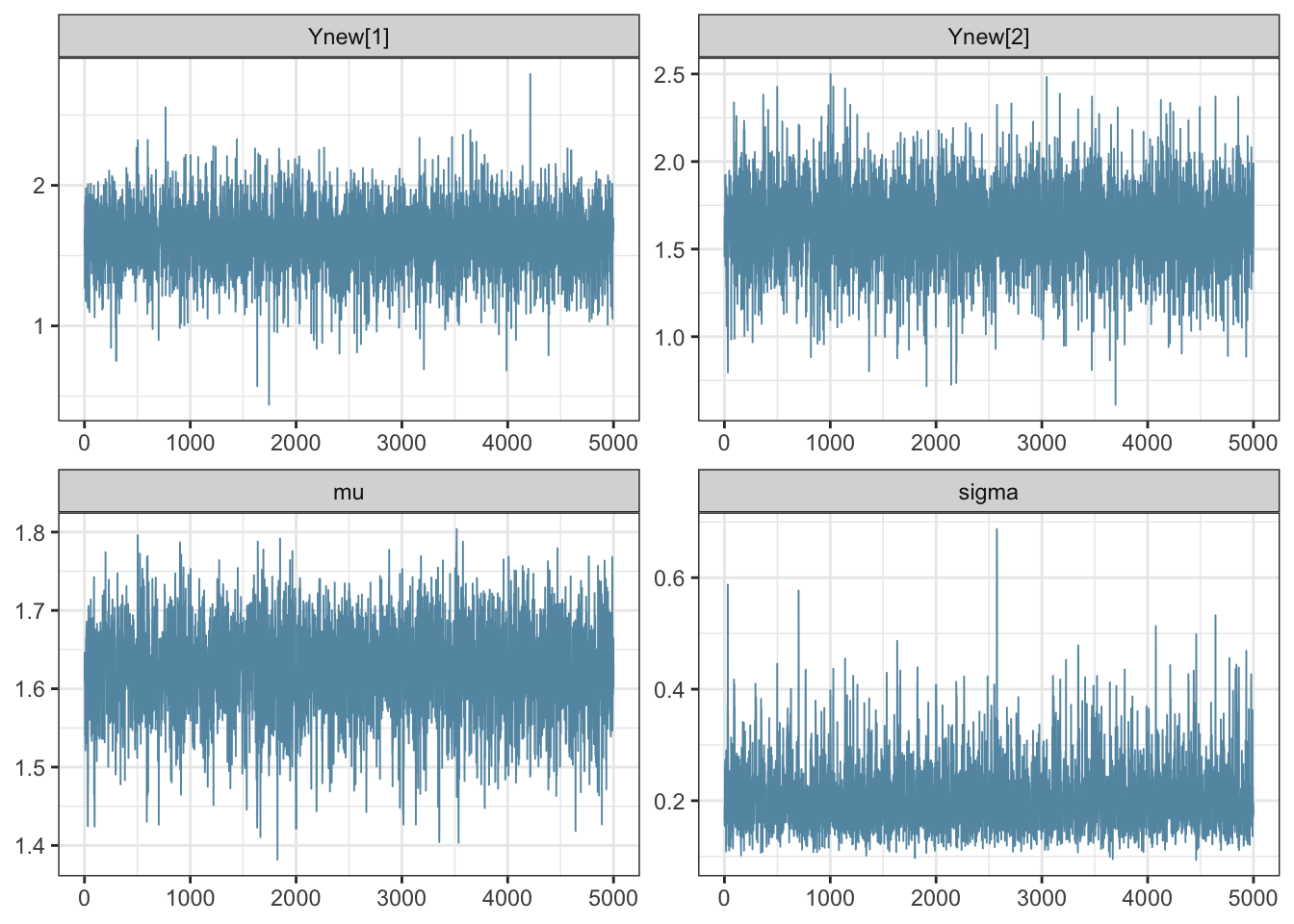
Figure 3.4: (ref:hier)
The following is similar to the caterpillar plot, but shows density functions.
bayesplot::mcmc_areas(fit, pars = vars(contains("Ynew"),"mu","sigma"),
                      prob_outer = 0.95)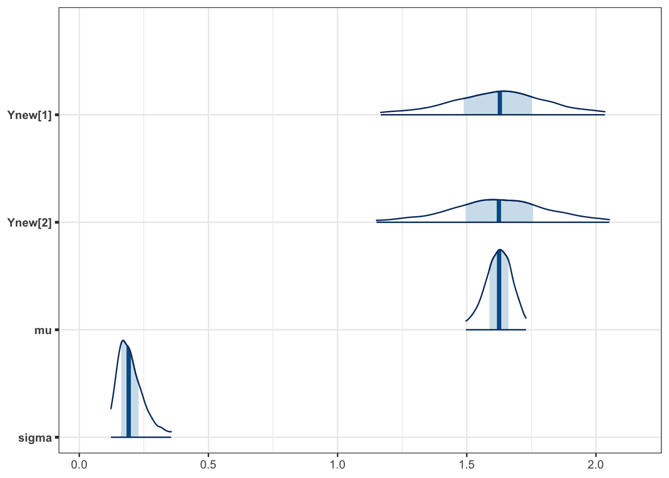
Figure 3.5: (ref:hier)
3.7.1.3 shinyStan
An interactive approach for exploring the results of the sampler is using the shinystan package (Gabry 2018), which launches a shiny application in your browser. To launch this, you would use the command:
ssfit <- shinystan::as.shinystan(fit)
shinyStan::launch_shinystan(ssfit)
3.8 No U-Turn Sampler (NUTS)
You might have noticed that the information about the Stan sampler we implemented in this section said
Samples were drawn using NUTS(diag_e).
This is because Stan does not actually use the base HMC algorithm that we have introduced, but an improvement to this known as the No U-Turn Sampler.
The base HMC algorithm requires the specification of a tuning parameter, \(T\), which controls how much ‘time’ the fictitious ball rolls around the parameter space before being stopped in each iteration. The choice of \(T\) is not an easy one. In Figure 3.6 we show the proposed path from our earlier bivariate Gaussian example, but the difference here is that in the right panel the ball was left for twice the amount of time as the first. Although more time was allowed for the ball to move around, it has actually ended up closer to its original location than the left example. This is because it did a U-turn.
The ideal implementation of HMC would be to choose a value for \(T\) that allows large moves to be made, such as the left example in Figure 3.6. We could attempt to identify the ideal \(T\) for a given analysis through pilot runs, similar to practices carried out for choosing the step variance in a random-walk MH. However, in a multi-modal parameter space, the ideal \(T\) that avoids U-turns would differ depending upon the current location in that space.
The NUTS algorithm is a modification of the original HMC algorithm that dynamically changes the tuning parameter \(T\) in each iteration to produce efficient results. We will not go into the details of this, but intuitively, the path is being simulated until the particle is no longer moving further away from the starting point, at which point it is stopped. The specifics of the implementation of this in practice require additional considerations for the sampler to be a valid MCMC sampler.
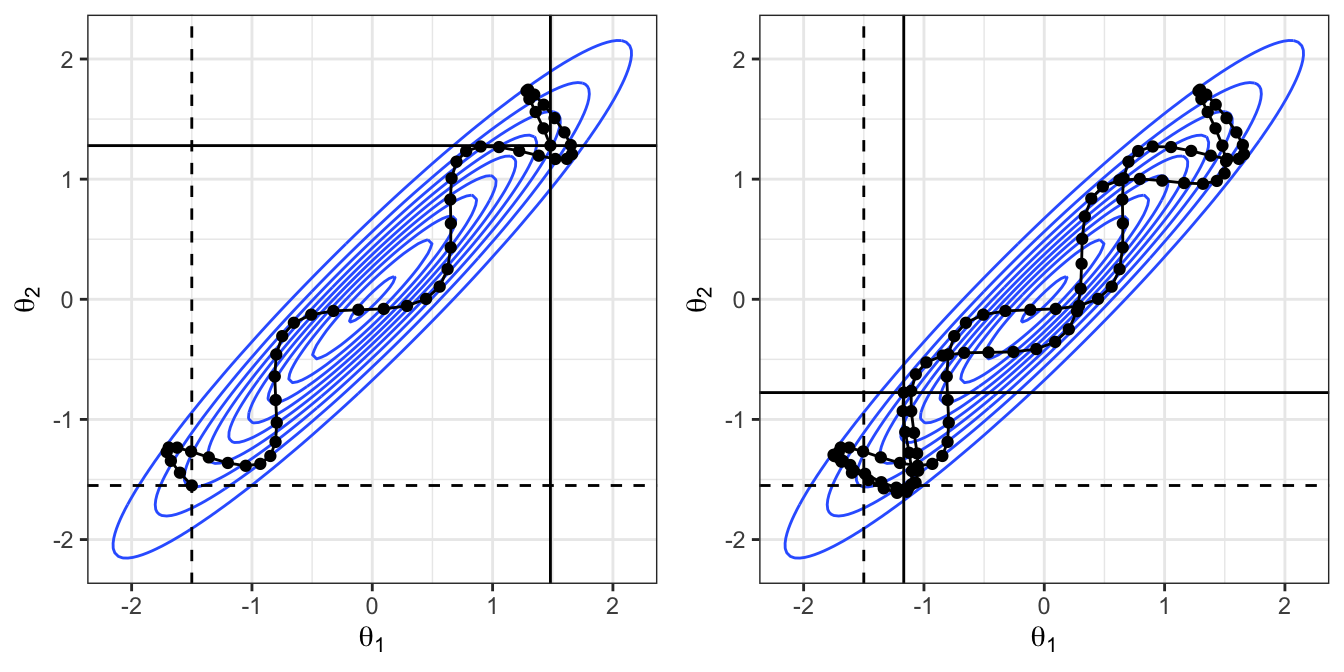
Figure 3.6: Given a starting location of (-1.5,-1.55) and an initial momentum of (-1,1), the leapfrog algorithm is implemented. Left: for 5 time-units. Right: for 10 time-units. The resulting path is shown with initial position highlight by the dashed line, and the final position highlighted by the solid line.
3.9 Further reading
Several online guides are available from the Stan home page:
- The User’s Guide has lots of examples for particular models. Try here if you know what model you want to fit.
- Stan Functions Reference includes sections describing probability distributions you might want to use and how to implement them in Stan.
- Stan Reference Manual includes information about writing Stan programs, in particular (Section 8) on the different types of code blocks.