Chapter 9 Coordinate ascent variational inference (CAVI)
\(\def \mb{\mathbb}\) \(\def \E{\mb{E}}\) \(\def \P{\mb{P}}\) \(\DeclareMathOperator{\var}{Var}\) \(\DeclareMathOperator{\cov}{Cov}\)
| Aims of this section |
|---|
| 1. Present one method for implementing variational inference: the CAVI algorithm. |
| 2. Demonstrate its application in a simple mixture modelling example. |
9.1 The CAVI algorithm
Given a mean-field family of approximate distributions, we can use the CAVI algorithm to maximise the ELBO. For an \(m\)-dimensional parameter \(\boldsymbol\theta\), the algorithm is as follows.
- Choose some initial mean-field approximation \[q(\boldsymbol\theta)=\prod_{i=1}^m q_i(\theta_i).\]
- Update each \(q_i\) in turn for \(i=1,\ldots,m\). Holding \(q_j(\theta_j)\) fixed for all \(j\neq i\), replace the current \(q_i\) in the mean-field approximation with \[\begin{equation} q_i(\theta_i)^* \propto \exp \left\lbrace \E_{q_{-i}} \left[\log p\left( \theta_i , \boldsymbol\theta_{-i}, x \right)\right]\right\rbrace. \tag{9.1} \end{equation}\]
- Repeat step 2 until the ELBO has converged.
The update for \(q_i\) in equation (9.1) is optimal, in that it gives the greatest increase in the ELBO. To see this, we consider the ELBO as a function of \(q_i\) only and write
\[ ELBO(q_i) = \E_{q_i}[\E_{q_{-i}} [\log p(\theta_i, \boldsymbol\theta_{-i},x)]] - \E_{q_i}[\log q_i(\theta_i)] + K, \] for some constant \(K\). This hold because of the independence in the mean-field approximation. Then, we note that
\[\begin{align} -KL(q_i ||q^*_i) &= -\E_{q_i}[\log q_i(\theta_i) - \log q^*_i(\theta_i)] \\ &=- \E_{q_i}[\log q_i(\theta_i)] + \E_{q_i}[\E_{q_{-i}} [\log p(\theta_i, \boldsymbol\theta_{-i},x)]] + C, \end{align}\] for some constant \(C\), so that \(ELBO(q_i)\) is equal to \(-KL(q_i ||q^*_i)\) plus some constant term. As \(KL(q_i ||q^*_i)\) is minimised by setting \(q_i = q^*_i\), this must maximise the ELBO as a function of \(q_i\).
Note there is some similarity with Gibbs sampling here. In Gibbs sampling, we iterate through the conditional distributions, drawing samples at each time. In CAVI, we again iterate through the dimensions, but we are now updating the distribution at each iteration, rather than sampling.
9.2 Example: Mixture of Gaussians
9.2.1 The observation model
Consider \(K\) mixtures of Gaussians, where each has a different mean \(\mu_i\) but a common variance of 1. We have \(n\) observations \(x_1,\ldots,x_n\), where each observation is distributed according to one of the \(K\) mixture components, so that \[x_i \sim N(\mu_{c_i},1),\] where \(c_i\) is the mixture assignment of observation \(i\). Note that we do not observe the \(c_i\), and \(c_i\in \lbrace 1,\ldots,K\rbrace\). This model therefore has the set of unknown parameters \(\boldsymbol{\theta}=\lbrace \boldsymbol\mu,\mathbf{c}\rbrace\): the \(K\) class means and the \(n\) class assignments. Note that we can also refer to the class assignments as \(\mathbf{C}_i\), associated with observation \(x_i\), which is a vector of length \(K\), where all entries are 0 except the \(c_i^\text{th}\), which is 1. This alternative treatment seems overly complex, but it will turn out to be useful for some algebra later.
Note that one might think of the class probabilities/proportions as being included in the uncertain quantities of interest: the uncertain population proportion belonging to class \(i\), for \(i=1,\ldots,K\). But this is not the focus here: our interest is in the uncertain class assignments \(c_i\) for each observation.
9.2.2 The prior
We assume that there is a global distribution that these component means independently arise from, so that the prior for the class means is \[\mu_i \sim N(0, \sigma^2),\] for \(i=1,\ldots,K\). We will assume that we know the hyperparameter \(\sigma^2\). In the following we will keep this hyperparameter general, and remember that it is a known constant.
The class assignment \(c_i\) of observation \(i\) is a categorical variable, taking one of the values \(1,\ldots,K\). We assume a prior for this which is a categorical distribution with equal weightings, i.e. \((1/K,\ldots,1/K)\).
9.2.3 The joint likelihood
This is a classic example for variational inference because the expression for \(p(\mathbf{x})\) is computationally burdensome, being exponential in the number of mixture components, \(K\). We can express the joint density as \[\log p(\boldsymbol{\theta},\mathbf{x})=\sum_{k=1}^K \log p(\mu_k)+\sum_{i=1}^n \left[\log p(c_i)+\log p(x_i|c_i,\mu_i)\right],\] where:
- \(p(\mu_k)\) is the Gaussian prior, where for each \(k\) they are identically distributed, having mean 0 and known variance \(\sigma^2\). We can write \(\log p(\mu_k)\propto -\frac{\mu_k^2}{2\sigma^2}\).
- \(p(c_i)\) is a categorical distribution describing the weightings/probability of each mixture component arising (all equal at \(1/K\)). It is easiest here to work with the vector form of this variable, \(\mathbf{C}_i\). Using our prior of equal weightings, this means \(p(\mathbf{C}_i)=(\frac{1}{K},\ldots,\frac{1}{K})\) for all \(i\) and \(\log p(C_{ik})=-\log K\). This is a constant with respect to our parameters of interest and so, as we are only interested in likelihoods up to proportionality when considering gradients, we can drop this contribution to the joint likelihood.
- \(p(x_i|c_i,\mu_i)\) is the Gaussian with mean \(\mu_{c_i}\) and variance \(1\). We are again going to make use of our vector \(\mathbf{C}_i\) here, as although it is intuitive to think of the mean as \(\mu_{c_i}\), it’s tricky to work with this. We have \[\log p(x_i|c_i,\mu_i)=\log \prod_{k=1}^K p(x_i|\mu_k)^{C_{ik}}=\sum_{k=1}^K C_{ik} \log p(x_i|\mu_k)\propto -\frac{1}{2}\sum_{k=1}^K C_{ik} (x_i-\mu_k)^2.\]
Combining all of the above, we can write \[\begin{equation} \log p(\boldsymbol{\theta},\mathbf{x}) \propto -\frac{1}{2\sigma^2}\sum_{k=1}^K \mu_k^2 - \frac{1}{2}\sum_{i=1}^n \sum_{k=1}^K C_{ik} (x_i-\mu_k)^2. \tag{9.2} \end{equation}\]
9.2.4 The mean-field family approximation
If we are to assume a mean-field approximation to this system, we need a family of distributions \[\begin{equation} q(\boldsymbol{\theta})=\prod_{k=1}^K q(\mu_k | m_k,s_k^2) \prod_{i=1}^n q(\mathbf{C}_i | \boldsymbol\phi_i), \tag{9.3} \end{equation}\] as we assume that our parameters are independent from one another.
We will assume that the class means \(\mu_k\) have Gaussian distributions, and so there are variational parameters \(m_k\) and \(s_k^2\) that describe the range of Gaussians within the variational family. It is common practice to assume that the approximate distribution of a continuous variable is Gaussian.
We will then assume a categorical distribution for the \(i^\text{th}\) observation’s class, which has a vector of \(K\) component weights/probabilities given by \(\phi_i\).
Again, note that we have one set of variational parameters \((m_k, s^2_k)\) per mixture component, and one set of variational parameters \(\boldsymbol\phi_i\) per observation, because we’re interested in the class membership of each observation here.
We can express our variational family as \[\begin{equation} \log q(\boldsymbol{\theta}) \propto \sum_{i=1}^n \sum_{k=1}^K \log \phi_{ik} - \frac{1}{2}\sum_{k=1}^K \left( \log(2\pi s_k^2)+ \frac{(\mu_k-m_k)^2}{s_k^2} \right). \tag{9.4} \end{equation}\]
You may notice that we have assumed the same functional form for our approximate distribution for \(\boldsymbol\theta|\mathbf{x}\) as we did for our prior \(\boldsymbol\theta\). This isn’t mandatory for variational inference, but is common. The variational parameter \(\boldsymbol\phi_i\) features in the prior as \((\frac{1}{K},\ldots,\frac{1}{K})\), and the parameters \(m_k\) and \(s_k^2\) feature as \(0\) and \(\sigma^2\), respectively, for all \(k\in1,\ldots,K\). It’s useful to compare the prior to posterior as part of our analysis.
9.2.5 CAVI
In this example, our \(q(\cdot)\in \mathcal{Q}\) is defined by the values of \(\mathbf{m},\mathbf{s}^2,\boldsymbol{\phi}_i\), so we are optimising the ELBO with respect to this set of variational parameters. An iteration of the optimisation process will involve updating each of \(m_1,\ldots,m_K,s_1^2,\ldots,s_K^2,\boldsymbol{\phi}_1,\ldots,\boldsymbol\phi_n\) in turn. This sounds like a lot, but we will see the update process of that in Equation (9.1) for each of \(m_k,s_k^2,\boldsymbol{\phi}_i\) simplifies down to a set of neat, short equations.
We have \[\begin{align} ELBO(q) =& \ \E_q \left[ \log p(\boldsymbol\theta,\mathbf{x})\right] - \E_q \left[ \log q(\boldsymbol\theta) \right] \\ \propto& -\frac{1}{2\sigma^2}\sum_{k=1}^K \E_q\left[\mu_k^2\right] - \frac{1}{2}\sum_{i=1}^n \E_q\left[\sum_{k=1}^K C_{ik} (x_i-\mu_k)^2\right] \\ &-\sum_{i=1}^n \sum_{k=1}^K \E_q\left[\log \phi_{ik}\right] + \frac{1}{2}\sum_{k=1}^K \E_q\left[ \log(2\pi s_k^2)+ \frac{(\mu_k-m_k)^2}{s_k^2} \right], \end{align}\]
We are going to derive in detail the update for \(\boldsymbol\phi_i\). We will then only give results for the update for \(m_k,s_k^2\); you can derive these results for yourself if you wish.
9.2.5.1 The CAVI update for the mixture class assignment
The variational family for each class assignment \(\mathbf{C}_i\) is a categorical distribution of the form \[ q(\mathbf{C}_i|\boldsymbol\phi_i) = \prod_{j=1}^K \phi_{ij}^{C_{ij}}, \] so that \[\begin{equation} \log q(\mathbf{C}_i|\boldsymbol\phi_i) = \sum_{i=1}^K C_{ij}\log \phi_{ij} \tag{9.5} \end{equation}\]
The CAVI update for \(\boldsymbol\phi_i\) means that we are updating just part of our variational family. Recall that we implement CAVI parameter by parameter because of our independence assumption. So our full variational distribution is that in Equation (9.3), and our update for \(\boldsymbol\phi_i\) means we are updating the part of the variational distribution \(q(\mathbf{C}_i|\boldsymbol\phi_i)\). From Equation (9.1) we need to set \[q(\mathbf{C}_i|\boldsymbol\phi_i)^* \propto \exp \left\lbrace \E_{-\boldsymbol\phi_i} \left[\log p\left( \boldsymbol{\phi}_i , \boldsymbol\theta_{-\boldsymbol{\phi}_i}, \mathbf{x} \right)\right]\right\rbrace.\] As this is a function of \(\boldsymbol\phi_i\), we only need to take all the elements in our expression for \(p\left( \boldsymbol{\phi}_i , \boldsymbol\theta_{-\boldsymbol{\phi}_i}, \mathbf{x} \right)\) in Equation (9.2) that involve \(\boldsymbol\phi_i\) (i.e. we only consider up to proportionality). This is therefore \[\begin{align} q(\mathbf{C}_i|\boldsymbol\phi_i)^* &\propto \exp \left\lbrace \E_{-\boldsymbol\phi_i} \left[ -\frac{1}{2}\sum_{k=1}^K C_{ik} (x_i-\mu_k)^2\right]\right\rbrace \\ &= \exp \left\lbrace -\frac{1}{2}\sum_{k=1}^K C_{ik}\E_{-\boldsymbol\phi_i}\left[ x_i^2-2x_i\mu_k+\mu_k^2\right]\right\rbrace \\ &\propto \exp \left\lbrace \sum_{k=1}^K C_{ik}\left(x_i\E_{-\boldsymbol\phi_i}\left[\mu_k\right]-\frac{1}{2}\E_{-\boldsymbol\phi_i}\left[\mu_k^2\right]\right)\right\rbrace \\ &=\exp \left\lbrace \sum_{k=1}^K C_{ik}\left(x_im_k-\frac{m_k^2+s_k^2}{2}\right)\right\rbrace. \end{align}\]
We have simplified this expression as much as possible, but where does that leave us? Now we compare the expression above, with Equation (9.5) , and we set \[\phi_{ij} \propto \exp \left\lbrace x_im_k-\frac{m_k^2+s_k^2}{2}\right\rbrace.\]
9.2.5.2 The complete CAVI update
In summary, in an iterated update of the CAVI approach, we replace the current set of \(\boldsymbol\phi_1,\ldots,\boldsymbol\phi_n\) with the above expression, where \(m,s^2\) are the current values of these parameters. A complete iteration of CAVI will then involve updating \(m_1,\ldots,m_K\) given the current values of the remaining parameters, and then updating \(s_1^2,\ldots,s_K^2\) given the current values of the remaining parameters. We will not show the derivation, but these updates are: \[\begin{align} m_k &= \frac{\sum_{i=1}^n \phi_{ik}x_i}{\frac{1}{\sigma^2} + \sum_{i=1}^n \phi_{ik}}, \\ s_k^2 &= \frac{1}{\frac{1}{\sigma^2} + \sum_{i=1}^n \phi_{ik}}. \end{align}\]
9.2.6 Implementing CAVI in R
We show CAVI in practice for an example of a mixture of 3 Gaussians. We generate some observations:
# create observations
true_mu <- c(-2,0,3)
sigma <- 1
n <- 1000
K <- 3
true_c <- sample(1:K, n, replace = T)
x <- rnorm(n, true_mu[true_c], 1)
Then run the CAVI algorithm:
n_iter <- 1000
stored_m <- matrix(NA, nrow = n_iter, ncol = K)
# initial values
m <- rnorm(K)
s <- rep(1, K)
phi <- matrix(NA, nrow = n_iter, ncol = K)

# CAVI
for (j in 1:n_iter) {
  for(i in 1:n) {
    phi[i, ] <- exp(m*x[i] - (m^2+s)/2)
    # normalise phi as they are supposed to sum to 1
    phi[i, ] <- phi[i, ] / sqrt(sum(phi[i, ])^2)
  }
  for(k in 1:K) {
    m[k] <- sum(phi[ , k] * x) / (1/sigma^2 + sum(phi[ , k]))
    s[k] <- 1 / (1/sigma^2 + sum(phi[ , k]))
  }
  # keep track of the m's each iteration to see convergence
  stored_m[j, ] <- m
}
Results of this analysis are plotted in Figures 9.1 and 9.2. Remember that the outcome of CAVI is a set of optimal values for \(m_k,s_k^2,\boldsymbol\phi_i\), and these optimal values define the joint distribution of \(\boldsymbol\theta\) that is used as an approximation to the posterior.
We have observations \(x\) that arise from one of 3 Gaussians, and the true data is shown in the left panel of Figure 9.1, showing the general range of \(x\) values produced from each group classification. In the right panel of Figure 9.1 we show the most probable group classification, defined for each observation \(x_i\) as the most probable class from \(\boldsymbol\phi_i=(\phi_{i1},\phi_{i2},\phi_{i3})\). This is a fairly easy classification problem, as you can see that the observations from the three groups are fairly well separated, with only a small overlap. The VI classification has clear cut boundaries between the three groups when we look at the most probable classifications, but note that if we were to delve into the \(\boldsymbol\phi_i\) for an observation that is on the boundary between groupings (i.e. an outlier in the box plots in the left panel), there will likely be uncertainty in the predicted classification. For example, observation \(13\) had value \(x_{13}=-0.848\) and was simulated from group \(1\). This value is in the tail of that Gaussian distribution, and the estimate of the class probabilities was \((0.457, 0.542, 6.1\times 10^{-4})\), so although it was deemed most likely to have arisen from group 2 (incorrectly), we can see it was almost equally deemed to be from groups 1 or 2.
We can also produce a confusion matrix with the caret package. We have the true classes in true_c, and we extract the predictions as follows:
most_lik <- rep(NA, n)
for(i in 1:n) {
  most_lik[i] <- which(phi[i, ] == max(phi[i, ]))
}
Then we do
caret::confusionMatrix(as.factor(true_c),
                       as.factor(most_lik))$table
## Reference
## Prediction 1 2 3
## 1 254 1 56
## 2 52 26 264
## 3 0 328 19In Figure 9.2 we show the results of the group means, the \(\mu_1,\mu_2,\mu_3\). The distributions are the results from CAVI. Recall that CAVI gives the optimal \(m_k\) and \(s_k^2\) that define the approximate distribution of independent Gaussians for the \(\mu_k\). The true mixture means are shown with dashed lines, and we can see these have been replicated well by this analysis. Something to note it that this approach cannot include correlations between the parameters. If the distribution for \(\mu_1\) was to be lowered, then this would obviously affect the group classification probabilities \(\boldsymbol\phi_i\), i.e. there is correlation in our model system that we expect to exist that we cannot estimate. This is important to always bear in mind with VI.
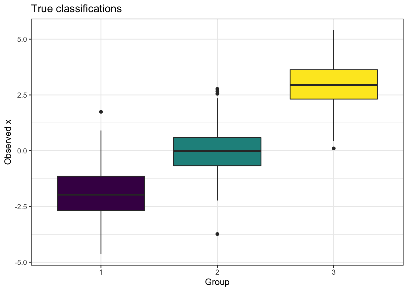
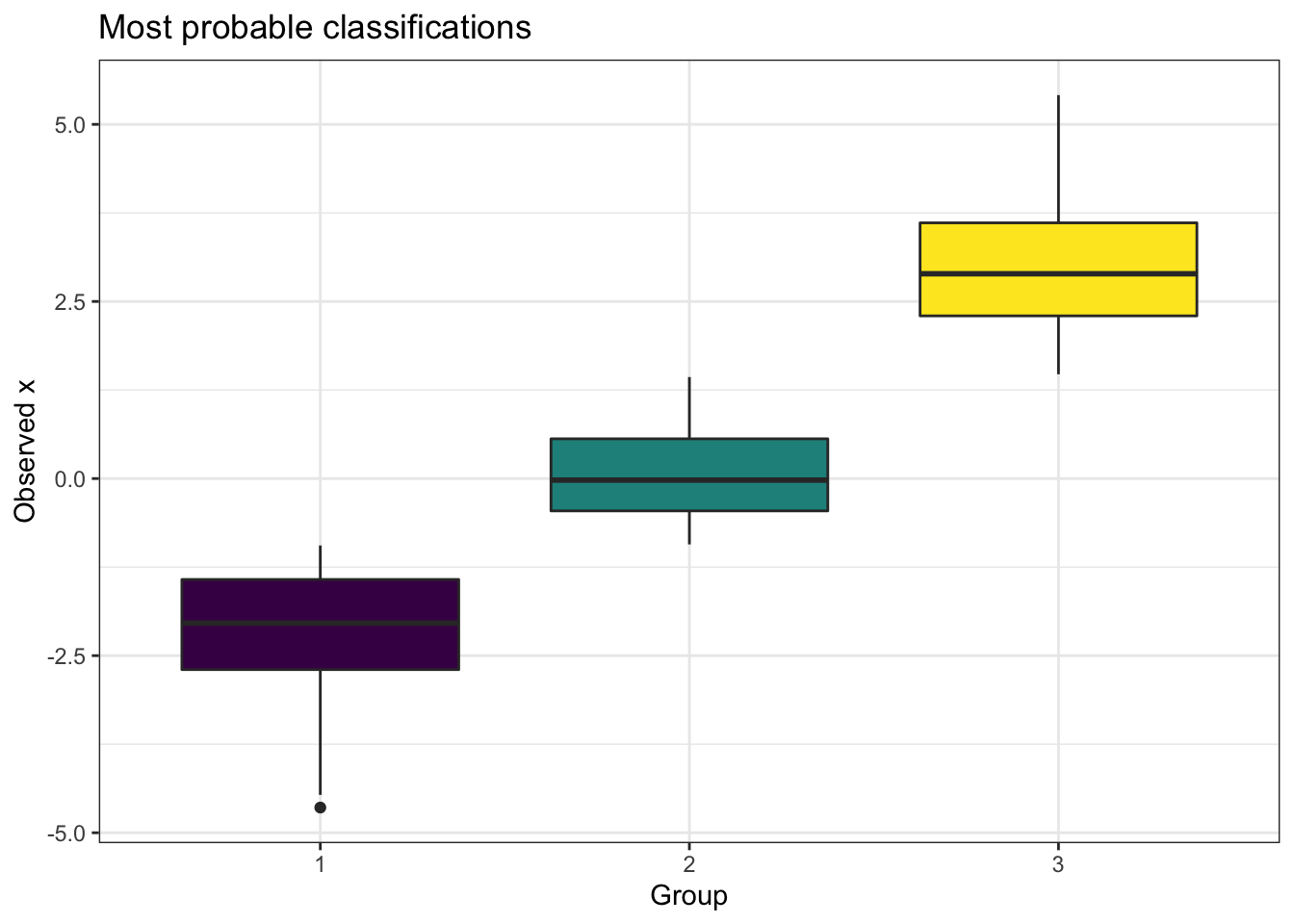
Figure 9.1: The distribution of observations, split by the true underlying mixture group classification (left panel) and the most probable classification from applying CAVI (right panel).
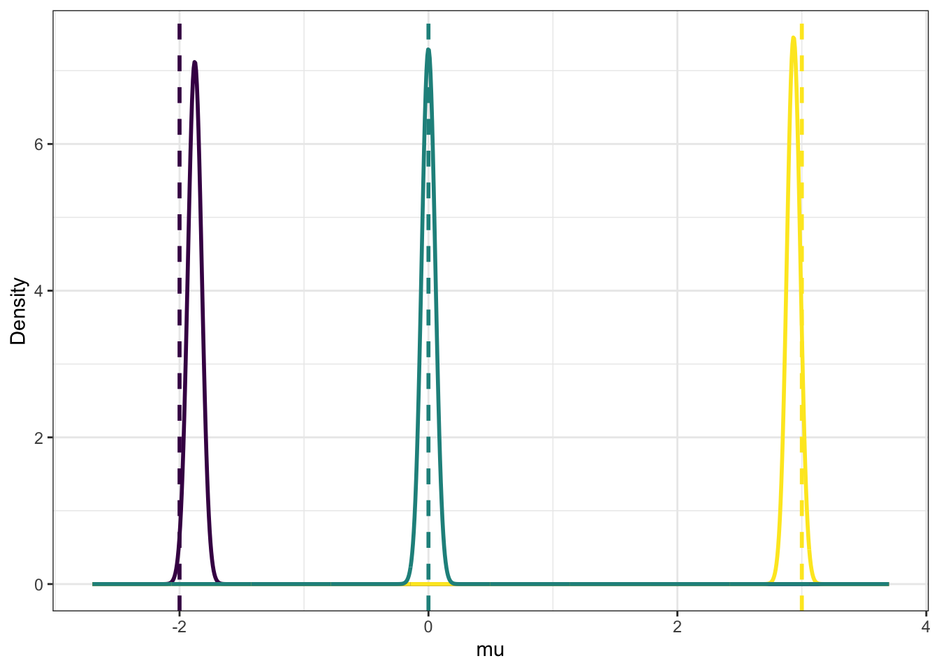
Figure 9.2: The approximate posterior distributions of the mixture means from CAVI (solid), along with the true means used for the simulation (dashed).