Chapter 5 Multiple imputation for missing data
\(\def \mb{\mathbb}\) \(\def \E{\mb{E}}\) \(\def \P{\mb{P}}\) \(\def \R{\mb{R}}\) \(\DeclareMathOperator{\var}{Var}\) \(\DeclareMathOperator{\cov}{Cov}\)
| Aims of this chapter |
|---|
| 1. Introduce and discuss statistical issues with missing data. |
| 2. Understand the multiple imputation approach. |
3. Implement and interpret the results of multiple imputation in
practice using the R package mice. |
5.1 Introduction
It is common to encounter data sets where some of the values are missing, for example, in a sample survey if a respondent does not answer all the questions, or if a process for recording data wasn’t working on a particular day. Some scenarios are as follows.
- Missing data we may choose to ignore.
Consider, for example, the airquality data frame in R:
head(airquality)## Ozone Solar.R Wind Temp Month Day
## 1 41 190 7.4 67 5 1
## 2 36 118 8.0 72 5 2
## 3 12 149 12.6 74 5 3
## 4 18 313 11.5 62 5 4
## 5 NA NA 14.3 56 5 5
## 6 28 NA 14.9 66 5 6Each NA indicates a missing value. If we fit a linear model in R using
these data, R will ignore any row with a missing value. This is
sometimes referred to as a complete case analysis.
- Censored data
In a clinical trial, we may observe ‘survival data’: the time \(T\) taken for some event to occur for a patient. Suppose, for example, a trial lasts for two years, and that for a particular patient, the event hasn’t occurred by the end of the trial. For this patient, we have a censored observation: we only know \(T>2\); the actual value of \(T\) is not observed. Here, we can incorporate this observation into our analysis through appropriate specification of the likelihood function. The contribution to the likelihood from this patient’s observation would be of the form \(P(T>2|\theta)\), rather than a density \(f_T(t|\theta)\), had we observed \(T=t\).
- Bias
In a sample survey, the probability of a participant answering a question may depend on the answer the participant would give. For example, in a political opinion poll, participants with particular views may be less likely to answer certain questions. This is perhaps the hardest type of missing data to deal with; ignoring it could lead to biased results. We may have to make strong modelling assumptions, or seek additional data that would help us understand potential biases.
In this chapter, we will study one particular technique for dealing with missing data: multiple imputation. We’ll consider this from a Bayesian perspective, so the aim will be to derive posterior distributions in situations with missing data.
5.2 Example: nhanes data
We will be using an example with a dataset nhanes from the mice
package (van Buuren and Groothuis-Oudshoorn 2011), which comprises 25 observations of 4 variables. An extract of
this data is shown in Table 5.1, which includes a
number of missing cells.
| age | bmi | hyp | chl |
|---|---|---|---|
| 1 | NA | NA | NA |
| 2 | 22.7 | 1 | 187 |
| 1 | NA | 1 | 187 |
| 3 | NA | NA | NA |
| 1 | 20.4 | 1 | 113 |
| 3 | NA | NA | 184 |
| 1 | 22.5 | 1 | 118 |
| 1 | 30.1 | 1 | 187 |
| 2 | 22.0 | 1 | 238 |
| 2 | NA | NA | NA |
Using the mice package, we can investigate the missing data pattern of
our dataset. Our classic tools for exploratory data analysis do still
stand and are somewhat informative, such as summary will tell us the
number of missing observations per variable. However, the pattern
between variables does not come across here:
summary(mice::nhanes)## age bmi hyp chl
## Min. :1.00 Min. :20.40 Min. :1.000 Min. :113.0
## 1st Qu.:1.00 1st Qu.:22.65 1st Qu.:1.000 1st Qu.:185.0
## Median :2.00 Median :26.75 Median :1.000 Median :187.0
## Mean :1.76 Mean :26.56 Mean :1.235 Mean :191.4
## 3rd Qu.:2.00 3rd Qu.:28.93 3rd Qu.:1.000 3rd Qu.:212.0
## Max. :3.00 Max. :35.30 Max. :2.000 Max. :284.0
## NA's :9 NA's :8 NA's :10In the below, we use md.pattern() to obtain this information, which
can both print out this missing pattern, and display it with an image,
as given in Figure 5.1.
Each column represents one variable in the data, but each row is not a subject. Each row is a missingness pattern across the set of variables, that is present in the data. The left column of figures gives the number of subjects with that missing pattern, and the right column of figures gives the number of missing data that pattern involves (i.e. how many red squares are in that row). The bottom row of numbers therefore counts how many subjects have missing data for each variable.
mice::md.pattern(mice::nhanes)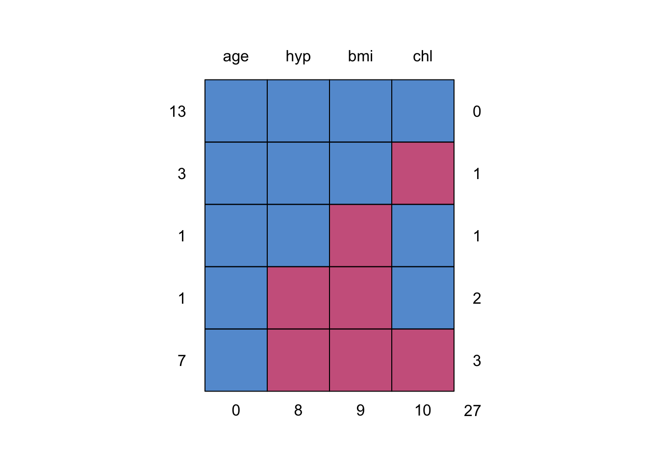
Figure 5.1: Missing data pattern of the nhanes dataset.
##    age hyp bmi chl
## 13   1   1   1   1  0
## 3    1   1   1   0  1
## 1    1   1   0   1  1
## 1    1   0   0   1  2
## 7    1   0   0   0  3
##      0   8   9  10 27
For the nhanes data, we have 13 subjects with full information, 4
subjects who have one variable out of the four missing, 1 subject with
two variables missing, and finally 7 subjects who have the same set of
the three variables missing. Note that all 25 subjects have observations
of the variable age.
5.3 Mechanisms of missingness
Suppose we have data \(Y = (y_{ij})\) given by the \(n \times k\) matrix, which will typically contain information about \(k\) variables from \(n\) subjects. We distinguish the pattern of the missing data by introducing the missing-data indicator matrix, \(R = (r_{ij})\), such that \(r_{ij}=1\) if \(y_{ij}\) is missing and \(r_{ij}=0\) if \(y_{ij}\) is present.
The pattern of missing data arises due to the mechanism of missingness. This is characterised by the conditional distribution of \(R\) given \(Y\) and two sets of parameters:
- \(\theta\): the parameters of interest, i.e. parameters in a likelihood \(f(Y|\theta)\);
- \(\phi\): nuisances parameters that are related to the missing data mechanism only, e.g. a probability of non-response in a sample survey.
In the following discussion, we will assume \(\theta\) and \(\phi\) are independent, and that conditional on \(Y\), we have independence between \(R\) and \(\theta\): given \(Y\), missingness is not dependent on the parameters in the distribution of \(Y\). We will therefore consider missingness mechanisms in terms of the distribution \(f(R|Y, \phi)\).
Three possible mechanisms are as follows.
5.3.1 Missing completely at random (MCAR)
Missingness does not depend on the value of the data, so \[f(R | Y, \phi) = f(R | \phi),\] for all \(Y,\phi\). This is the ideal situation. Note that this name is slightly confusing—the pattern of missing data given by \(R\) need not be random, but merely that it is independent of the data values themselves.
5.3.2 Missing at random (MAR)
Missingness depends only on the components of \(Y\) that are observed, denoted \(Y_\text{obs}\), and not on the components that are unobserved, denoted \(Y_\text{mis}\). So \[f(R | Y, \phi) = f(R | Y_\text{obs}, \phi),\] for all \(Y_\text{mis},\phi\). Here, the probability of a data point being missing can depend on the value of other variables that are not missing. For example, in a questionnaire there may be a question on salary that older age groups are more likely to not answer in comparison with younger age groups.
Note that MCAR implies MAR.
5.3.3 Not missing at random (NMAR)
Missingness can depend both on the missing and observed variables, so that \(f(R | Y, \phi)\) cannot be simplified. For example, respondents to a questionnaire may be more likely to leave a question on salary unanswered dependent upon their actual salary. This is the hardest mechanism of missing data to handle and can lead to serious biases.
5.4 Ignoring information about missingness
When we have missing data, the observed data should be thought of as both \(Y_\text{obs}\) and \(R\): the target posterior is \(f(\theta|Y_\text{obs}, R)\). We can ignore \(R\) if we assume that the data are missing at random (and hence also if the data are MCAR). For the joint posterior distribution of \(\theta, \phi\) we have
\[\begin{align} f(\theta,\phi | Y_\text{obs},R)&\propto \pi(\theta)\pi(\phi)f(Y_\text{obs},R|\theta, \phi),\\ &=\pi(\theta)\pi(\phi)f(Y_\text{obs}|\theta)f(R|Y_\text{obs}, \phi), \end{align}\] assuming the data are MAR. Hence for the marginal posterior of \(\theta\) we have \[ f(\theta|Y_\text{obs},R)\propto\pi(\theta)f(Y_\text{obs}|\theta), \] i.e. the posterior obtained if we ignore \(R\).
5.5 Inference via imputation
From now on, we will assume our data are MAR, so that \(R\) can be ignored.
Returning to the nhanes data, suppose we want to fit a regression
model with bmi as the dependent variable, and the other three
variables as the independent variables. Amongst the missing data, we
note one observation where bmi is observed, but chl is not:
mice::nhanes[24, ]## age bmi hyp chl
## 24 3 24.9 1 NAShould observations like this be ignored? As age and hyp were still
observed, wouldn’t there still be some information about the
relationship between dependent and independent variables from this
observation? In general, we may have a dataset where the proportion of
complete cases (observations with no missing variables) is relatively
small; if we only conduct a “complete case analysis” (where any
incomplete rows are discarded), we may be ignoring a lot of data.
Here, we define
- \(Y_\text{obs}\): all the observed individual observations, including any observed variables within rows containing missing data.
- \(Y_\text{mis}\): all the individual missing observations. (Together, \((Y_\text{obs}, Y_\text{mis})\) would give a complete data frame in R).
- \(\theta\): the model parameters of interest.
If we are to make use of all the data we have, we want to derive \(f(\theta|Y_\text{obs})\). But this will involve a likelihood \(f(Y_\text{obs}|\theta)\) that we can’t easily write down (how would we fit a linear model where some of the independent variables are missing?) The main idea of multiple imputation is to derive the posterior via
\[ f(\theta|Y_\text{obs}) = \int f(\theta|Y_\text{obs}, Y_\text{mis})f(Y_\text{mis}|Y_\text{obs})dY_\text{mis} \] The posterior \(f(\theta|Y_\text{obs}, Y_\text{mis})\) is the posterior of \(\theta\) given a complete data set, and so will be easier to deal with. We do, however, have a new problem, which is to consider a distribution of the missing data conditional on the observed data; we discuss this later.
Rather than trying to evaluate the integral analytically, we will use a Monte Carlo approach. In outline:
- we sample a set of missing data \(Y_\text{mis}^{(i)}\);
- we derive a posterior \(f(\theta|Y_\text{obs}, Y_\text{mis}^{(i)})\);
- we repeat steps (1) and (2) \(m\) times, and then average over our distributions \(f(\theta|Y_\text{obs}, Y_\text{mis}^{(1)}), \ldots f(\theta|Y_\text{obs}, Y_\text{mis}^{(m)}).\).
In effect, we are approximating the posterior of interest with \[f(\theta \ | \ Y_\text{obs}) \approx \frac{1}{m} \sum_{i=1}^m f(\theta \ | \ Y_\text{mis}^{(i)}, Y_\text{obs}),\] where \(Y_\text{mis}^{(i)} \sim f(Y_\text{mis} \ | \ Y_\text{obs})\).
The process of filling in the missing values is known as imputation, and because we do this multiple times, we refer to it as multiple imputation.
5.5.1 Further simplifications
Although deriving \(f(\theta|Y_\text{obs}, Y_\text{mis}^{(i)})\) is simpler than deriving \(f(\theta|Y_\text{obs})\), it still may be difficult, or involve substantial computational effort. We may choose to make two further simplifications:
- Instead of obtaining the full posterior distribution \(f(\theta \ | \ Y_\text{obs})\), we may just obtain the posterior mean and variance of \(\theta\), using only \(E(\theta \ | \ Y_\text{mis}^{(i)}, Y_\text{obs})\) and \(Var(\theta \ | \ Y_\text{mis}^{(i)}, Y_\text{obs})\) for \(i=1,\ldots,m\)
- We may choose to obtain quick approximations of \(E(\theta \ | \ Y_\text{mis}^{(i)}, Y_\text{obs})\) and \(Var(\theta \ | \ Y_\text{mis}^{(i)}, Y_\text{obs})\), for example (in a linear models setting) using a least squares estimate to approximate \(E(\theta \ | \ Y_\text{mis}^{(i)}, Y_\text{obs})\) and the associated standard error (squared) to approximate \(Var(\theta \ | \ Y_\text{mis}^{(i)}, Y_\text{obs})\).
5.6 Pooling multiple imputations
Suppose we have already we have already obtained \(m\) imputed datasets \((Y_\text{mis}^{(1)}, Y_\text{obs}), \ldots, (Y_\text{mis}^{(m)}, Y_\text{obs})\). We will use the simplification of obtaining approximate expressions for the posterior mean and variance \(\theta|Y_\text{obs}\); we will not attempt to derive the full posterior \(f(\theta|Y_\text{obs})\)
We estimate \(E(\theta|Y_\text{obs})\) by noting that \[ \E(\theta \ | \ Y_\text{obs}) = \E(\E(\theta \ | \ Y_\text{mis}, Y_\text{obs}) \ | \ Y_\text{obs}) \] and then using the estimate \[\begin{equation} \bar{\theta} := \frac{1}{m}\sum_{i=1}^m \hat{\theta}^{(i)}, \tag{5.1} \end{equation}\] where \[ \hat{\theta}^{(i)} = \E(\theta \ | \ Y_\text{mis}^{(i)}, Y_\text{obs}) \]
In the above, the first line uses the tower property of expectation. This equality says that the posterior mean is the average of the posterior means over repeatedly imputed data. The approach for combining the results of multiple imputation therefore arises by approximating the average by a sample mean of the estimator from our \(m\) imputations.
We estimate \(\var(\theta|Y_\text{obs})\) by first noting that \[ \var(\theta \ | \ Y_\text{obs}) = \E(\var(\theta \ | \ Y_\text{mis}, Y_\text{obs}) \ | \ Y_\text{obs}) + \var(\E(\theta \ | \ Y_\text{mis}, Y_\text{obs}) \ | \ Y_\text{obs}) , \] and then using the estimate
\[\begin{equation} T := \bar{U} + \left(1 + \frac{1}{m} \right)B, \tag{5.2} \end{equation}\] where \(\bar{U}\) is an estimate of \(\E(\var(\theta \ | \ Y_\text{mis}, Y_\text{obs}) \ | \ Y_\text{obs})\), given by \[ \bar{U}:= \frac{1}{m}\sum_{i=1}^m U^{(i)}, \quad U^{(i)}:=\var(\theta \ | \ Y_\text{mis}^{(i)}, Y_\text{obs}), \] and \(B\) is an estimate of \(\var(\E(\theta | Y_\text{mis}, Y_\text{obs}) | Y_\text{obs})\), given by \[ B:=\frac{1}{m-1} \sum_{i=1}^m \left(\hat{\theta}^{(i)} - \bar{\theta} \right)^2, \] and the factor \((1 + 1/m)\) is a correction for bias, the details of which we won’t consider here.
Writing \[\begin{equation} T = \bar{U} + B + \frac{B}{m}, \end{equation}\] we can summarise this as the posterior uncertainty of \(\theta\) comprising of three sources:
- The uncertainty caused by the fact that we are taking a sample of observations \(Y\) and estimating \(\theta\) from this. This is the uncertainty that we would always have surrounding an estimate from complete data, as \(Y\) is still only a sample and not the entire population of interest. This contribution is \(\bar{U}\).
- The uncertainty caused by the missing data. This contribution to the uncertainty is given by \(B\). Each imputed dataset represents a sample from the possible range of \(Y_\text{mis}\), so \(B\) is the variability in the parameter estimates resulting from the range of possible missing data values.
- The uncertainty caused by the fact that we have only implemented \(m\) imputed datasets and not the actual full set of possible \(Y_\text{mis}\). The contribution to the uncertainty from this aspect is \(\frac{B}{m}\).
Because any analysis will contain uncertainty of the type described in point (1), it is useful for us to evaluate the uncertainty that is arising because of the missing data and our imputation efforts. The proportion of the variance attributable to missing data and imputation out of the total variance can be expressed as \[\lambda_m := \frac{\left(1 + \frac{1}{m} \right)B}{\bar{U}+\left(1 + \frac{1}{m} \right)B}.\]
5.7 Simple example
We have the data in Table 5.2, which contains the three variables \(Y, X_1, X_2\), and there is one missing observation of \(X_1\).
| Y | X1 | X2 |
|---|---|---|
| 2.86 | 1.78 | 0.02 |
| 5.77 | 2.39 | 2.52 |
| 0.24 | -2.68 | 1.06 |
| 2.71 | -0.11 | 0.61 |
| -3.67 | NA | -1.67 |
| -2.99 | 1.59 | -2.26 |
The aim of this analysis is to build a regression model to predict \(Y\) from the two remaining variables \[Y_i=\beta_0+\beta_1 X_{1i}+\beta_2 X_{2i}+\epsilon_i,\] where \(\epsilon\sim N(0, \sigma^2)\).
5.7.1 Multiple imputation by hand
The multiple imputation work-flow consists of three steps:
- Imputing \(Y^{(1)},\ldots,Y^{(m)}\) from \(f(Y_\text{mis} | Y_\text{obs})\);
- Calculating the statistic of interest from the imputations, \(\hat{\theta}_1,\ldots,\hat{\theta}_m\); and
- Combining the imputations as \(\bar{\theta}\).
We have not yet discussed sophisticated methods for imputing datasets. For now, we will use a
simple imputation method that imputes a missing value as equal to a
randomly selected observation from that variable. In this example, this corresponds to a simple choice for the distribution \(f(Y_\text{mis} | Y_\text{obs})\), in which the missing data (a single missing value of X1) has a discrete uniform distribution, constructed from the observed values of X1.
Our statistic of interest here will be the estimates of the parameters \(\beta_0,\beta_1,\beta_2\). We will therefore store the estimate of these coefficients by fitting the proposed linear model to each imputed dataset. This forms our \(\hat{\theta}_1,\ldots,\hat{\theta}_m\).
For our estimates of uncertainty—see Equation
(5.2)—we will also need the variance of our
parameter estimates. For a linear model we access the covariance matrix
with vcov(). For simplicity here, we’ll just store the diagonal
elements of these and not consider the covariances between the
parameters.
Our imputation ‘by hand’ is given by the below (note that this has not been optimised in any way, but rather written for clarity of the process):
m <- 30
imputations <- rep(NA, m)
# store the imputed coefficients beta0, beta1, beta2
theta <- matrix(NA, nrow = m, ncol = 3)
# store the variance of each coefficient
V <- matrix(NA, nrow = m, ncol = 3)

for (i in 1:m) {

  imp <- sample(simple_data$X1[!is.na(simple_data$X1)], 1)
  complete_data <- simple_data
  complete_data$X1[is.na(complete_data$X1)] <- imp
  imputations[i] <- imp

  fit <- lm(Y ~ X1 + X2, data = complete_data)
  theta[i, ] <- coef(fit)
  V[i, ] <- diag(vcov(fit))
}
In the above we have implemented 30 imputations. An extract of the imputed parameter estimates \(\hat{\theta}^{(1)},\ldots,\hat{\theta}^{(30)}\) is given here, with the three columns being for \(\beta_0,\beta_1,\beta_2\), respectively. Note that some of these rows are the same—this is because our simple imputation method meant that our single missing value was randomly chosen from the five observations of that variable, so we know there will be repetitions in our imputations.
head(theta)## [,1] [,2] [,3]
## [1,] 0.2980052 0.4800095 1.996850
## [2,] 0.2911767 0.5745578 1.974844
## [3,] 0.4016995 0.6943554 1.871238
## [4,] 0.2980052 0.4800095 1.996850
## [5,] 0.4016995 0.6943554 1.871238
## [6,] 0.2911767 0.5745578 1.974844We pool our estimates to obtain \(\bar{\theta}\) by taking the sample mean of the imputed parameter estimates:
(theta_bar <- colMeans(theta))## [1] 0.3840886 0.5867359 1.9124154We calculate the variance of the pooled estimate using Equation (5.2) as:
(theta_var <- colMeans(V) + (1 + 1/m) * diag(cov(theta)))## [1] 0.4666031 0.1300045 0.1601651We calculate the proportion of the variance due to the missing observation as:
(lambda <- ((1 + 1/m) * diag(cov(theta))) / theta_var)## [1] 0.05311199 0.03803215 0.07565886We don’t need to implement imputation by hand, and will be
using the package mice. The equivalent of our analysis here is
implemented by specifying the method as 'sample':
imp_mice <- mice(simple_data, m = 30, method = 'sample', print = F)
fit_mice <- with(imp_mice, lm(Y ~ X1 + X2))
(pool_mice <- pool(fit_mice))
## Class: mipo m = 30
## term m estimate ubar b t dfcom df
## 1 (Intercept) 30 0.4085576 0.4339769 0.030391099 0.4653810 3 1.864493
## 2 X1 30 0.5818886 0.1209822 0.004851643 0.1259956 3 1.920219
## 3 X2 30 1.8982188 0.1460214 0.014711458 0.1612232 3 1.810413
## riv lambda fmi
## 1 0.07236361 0.06748048 0.4508789
## 2 0.04143885 0.03979000 0.4301019
## 3 0.10410694 0.09429063 0.4708526Remember that these methods are stochastic, and so we do not expect to
achieve equal results between these two implements when the number of
iterations is the same. Let’s compare our output, however. The estimate
\(\bar{\theta}\) is given by estimate, The components of the uncertainty
of this estimate are given as ubar and b, with the overall variance
given by t. The proportion of the variance due to missingness is given
by lambda.
5.8 Imputing missing data: chained equation multiple imputation
In theory, to draw the imputations, we should specify a model, potentially involving some unknown parameters \(\phi\): \[ f(Y_\text{mis} | Y_\text{obs}, \phi), \] specify a prior distribution \(\pi(\phi)\), and then sample \(\phi\) from \(\pi(\phi)\) and \(Y_\text{mis}\) from \(f(Y_\text{mis} | Y_\text{obs}, \phi)\). This is likely to be difficult, particularly if we have multiple variables with missing information, such that we need to define a joint distribution of the missingness over all variables.
One again, we will make some simplifications.
- We will propose a missingness process on a per-variable basis, conditional on the remaining variables. For example, if we have three variables \(X_1,X_2,X_3\), we will specify a missing process model of \[f(X_{\text{mis},1} \ | \ Y_\text{obs}, X_{\text{mis},2}, X_{\text{mis},3}, \phi),\] and likewise for \(X_2\) and \(X_3\).
- We will specify missing process models for each variable, with separate parameters and without considering whether they form a coherent joint distribution for all the missing variables. (We will need to rely on empirical evidence of whether doing this provides useful/appropriate imputations.)
A method we can use to implement this is called multiple imputation with chained equations, which is referred to as the MICE algorithm.
Suppose we have \(k\) variables, \(Y_1,\ldots,Y_k\). The observed data is given by \(Y_1^\text{obs},\ldots,Y_k^\text{obs}\), the missing data is \(Y_1^\text{mis},\ldots,Y_k^\text{mis}\) and ‘complete’ data will be referred to as \(Y_1,\ldots,Y_k\). For each variable \(j\in \lbrace1,\ldots,k\rbrace\) we specify the conditional imputation model \[f(Y_j^\text{mis} \ | \ Y_j^\text{obs}, Y_1, \ldots, Y_{j-1}, Y_{j+1},\ldots,Y_k,\phi_j).\] Note that we have a separate set of parameters \(\phi_j\) for each conditional imputation model.
The MICE algorithm imputes a single set of complete data, \(Y^{(i)}\). Starting from a random set of values for the missing data, the algorithm implements a number of Gibbs-style iterations to sample missing data from the conditional distributions that have been specified.
Recall that a Gibbs iteration implements the concept of sampling from a joint distribution of \(k\) variables by cycling through each of the dimensions in turn and updating them based on their full conditional distribution. Within the \(t^\text{th}\) iteration of Gibbs, if we are handling the \(j^\text{th}\) variable, then the conditional distribution that we would use to sample from would be \(f(Z_j \ | \ Z_1^t,\ldots,Z_{j-1}^t,Z_{j+1}^{t-1},\ldots,Z_{k}^{t-1})\). With MICE, we implement this same process. However, with multiple imputation, we often specify our conditional missing information distributions without considering whether these form a coherent joint distribution, which is why MICE is not necessarily a ‘true’ Gibbs sampler. Because of this, convergence is not guaranteed to a stationary distribution, but has been shown to produce useful imputations. The MICE algorithm is detailed in the following algorithm:
MICE Algorithm: To generate a single imputed dataset, \(Y^{(i)}\).
Initialise \(\dot{Y}_1^{0},\ldots,\dot{Y}_k^0\) by some simple approach, such as randomly sampling from the observed data \(Y_1^\text{obs},\ldots,Y_k^\text{obs}\).
Cycle through \(t=1,\ldots,M\) iterations of the following:
- Simulate \(\phi_1^t \sim f(\phi_1^t \ | \ Y^\text{obs},\dot{Y}_1^{t-1},\ldots,\dot{Y}_k^{t-1}),\) and set \[\dot{Y}_1^t \sim f(Y_1^\text{mis} \ | \ Y^\text{obs},\dot{Y}_2^{t-1},\ldots,\dot{Y}_k^{t-1},\phi_1^t).\]
- Simulate \(\phi_2^t \sim f(\phi_2^t \ | \ Y^\text{obs},\dot{Y}_1^t,\dot{Y}_2^{t-1},\ldots,\dot{Y}_k^{t-1}),\) and set \[\dot{Y}_2^t \sim f(Y_2^\text{mis} \ | \ Y^\text{obs},\dot{Y}_1^t,\dot{Y}_3^{t-1},\ldots,\dot{Y}_k^{t-1},\phi_2^t).\]
- Simulate \(\phi_3^t \sim f(\phi_3^t \ | \ Y^\text{obs},\dot{Y}_1^t,\ldots,\dot{Y}_3^t,\dot{Y}_4^{t-1},\ldots,\dot{Y}_k^{t-1}),\) and set \[\dot{Y}_3^t \sim f(Y_3^\text{mis} \ | \ Y^\text{obs},\dot{Y}_1^t,\dot{Y}_2^t,\dot{Y}_4^{t-1},\ldots,\dot{Y}_k^{t-1},\phi_3^t).\] \(\vdots\)
- Simulate \(\phi_k^t \sim f(\phi_k^t \ | \ Y^\text{obs},\dot{Y}_1^t,\ldots,\dot{Y}_{k}^{t}),\) and set \[\dot{Y}_k^t \sim f(Y_k^\text{mis} \ | \ Y^\text{obs},\dot{Y}_1^t,\ldots,\dot{Y}_{k-1}^{t},\phi_k^t).\]
Set \(Y^{(i)}_1,\ldots, Y^{(i)}_k=\dot{Y}^M_1,\ldots,\dot{Y}^M_k\).
Note that the MICE algorithm, although it involves \(M\) iterations, only produces a single imputed dataset. The intermediate simulated values, the \(\dot{Y}\), are discarded. To implement a multiple imputation work-flow, we therefore need to implement the MICE algorithm \(m\) times, independently from one another.
In summary, key points to note are
- this process will achieve our objective of obtaining multiple imputed datasets…
- …and will account for uncertainty in any parameters used to specify the conditional missing data distributions…
- …but at a cost that we may not have coherently specified a joint distribution for all the missing data, conditional on all the observed data. We need to recognise that our inferences will be approximate.
5.8.1 How many iterations?
MICE seems like a computationally intense process, because we need to implement \(M\) iterations, where we cycle through our \(k\) variables in each, to obtain a single imputed dataset. We repeat this whole process \(m\) times to obtain our multiple imputation set. In practice, the value of \(M\) is usually low (somewhere between 5 and 20 iterations). A number of studies have shown that this generally provides informative imputation datasets, because convergence of Gibbs-style samplers is fast when there is noise in the system and correlations are low. Situations we should be aware of in practice are when we have
- Very high correlations between the variables \(Y_i\);
- Missing data rates are high; and
- Constraints on parameters across different variables exist.
5.9 MICE example: the nhanes dataset
We previously introduced the nhanes dataset in this chapter and
explored its missingness pattern. Recall the structure of the data in
Table 5.1, and that we have variables age
(\(Y_\text{age}\)), bmi (\(Y_\text{bmi}\)), hyp (\(Y_\text{hyp}\)) and
chl (\(Y_\text{chl}\)). In this section we will implement the MICE
algorithm on this data. The goal of our analysis is going to be to
predict bmi from age and chl, i.e. we want to fit the regression
model
\[\begin{equation}
Y_{\text{bmi},i} \sim N(\beta_0 + \beta_\text{age} \ Y_{\text{age},i} + \beta_\text{chl} Y_{\text{chl},i} + \beta_\text{age*chl}Y_{\text{age},i}Y_{\text{chl},i}, \sigma^2),\tag{5.3}
\end{equation}\]
for \(i\in \lbrace 1,\ldots,25\rbrace\). Our parameters of
interest are therefore
\(\beta_0,\beta_\text{age},\beta_\text{chl},\beta_\text{age*chl},\sigma^2\).
Notice that we aren’t interested in the variable hyp for our
regression model, but we won’t remove this variable from our dataset
because we are interested in how it can be informative for imputing our
missing variables that do feature in the regression.
5.9.1 Complete case analysis
For completeness, let us fit a complete case analysis to this data to compare with out multiple imputation results.
nhanes_cc <- lm(bmi ~ chl * age, data = nhanes)This gives the following parameter estimates:
##
## Call:
## lm(formula = bmi ~ chl * age, data = nhanes)
##
## Residuals:
##     Min      1Q  Median      3Q     Max
## -6.8064 -0.9114  0.4048  2.4316  2.8864
##
## Coefficients:
##             Estimate Std. Error t value Pr(>|t|)
## (Intercept) 13.95690    8.54679   1.633   0.1369
## chl          0.11031    0.04370   2.524   0.0325 *
## age         -1.45829    5.77496  -0.253   0.8063
## chl:age     -0.01783    0.02557  -0.698   0.5031
## ---
## Signif. codes:  0 '***' 0.001 '**' 0.01 '*' 0.05 '.' 0.1 ' ' 1
##
## Residual standard error: 3.147 on 9 degrees of freedom
##   (12 observations deleted due to missingness)
## Multiple R-squared:  0.6482, Adjusted R-squared:  0.5309
## F-statistic: 5.528 on 3 and 9 DF,  p-value: 0.01982
5.9.2 Imputing the missing data
We use mice to impute 10 datasets, using regression models for the
missing data conditional distributions:
nhanes_imp <- mice(nhanes, m = 10, method = 'norm', print = F)The object created by using the mice function is a list containing a
wealth of information, including:
- The original, incomplete dataset,
data; - The imputed datasets,
imp(easily extracted for use with the functioncomplete()); - The number of imputations,
m; - A matrix of the relations used for the imputation model,
predictorMatrix. If all variables are used to impute all other variables, this will be a matrix of 1’s with 0’s on the diagonal; - Information on the mean of the generated missing data over the \(M\)
iterations that are internal to the MICE algorithm,
chainMean. This can be used to assess convergence of the Gibbs-style approach and whether \(M\) should be increased.
We can extract the imputed data and take a look at it, as shown in
Figure 5.2. This shows the fully observed data pairs
between bmi and age, bmi and chl, and chl and age with red
squares. Each set of coloured points is then one of the 10 imputed
datasets, and a regression line to highlight the general trend of these
is given. Note that these regression lines plotted are not the
regression lines used in the imputation algorithm, but are only the
regression of the resulting imputed dataset. We have shown bmi against
both age and chl as these are to be the elements of our analysis
regression. This exploratory plot suggests a relationship between these
variables, that remains similar throughout the range of imputed
datasets.
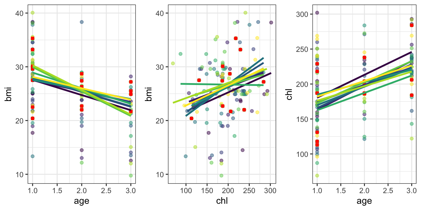
Figure 5.2: The imputed data using MICE for the nhanes dataset. For the three pairs of variables shown below, fully observed data are highlighted with red squares. Each of the 10 imputed datasets are shown by the varying colour scale of points. A regression line of each imputed set is shown—note that this is not related to the imputation regression model, but merely used to highlight the differences between the imputed datasets.
We can study the convergence of our MICE algorithm by using plot() on
the list produced by the mice() function. This plot, in Figure
5.3 has a row for each imputed variable (recall that
age is fully observed in our dataset so we have 3 variables being
imputed), and a column each for the mean and sd. Each plot contains \(m\)
lines, one for each imputation.
The points on the \(x\)-axis are the
iterations within the MICE algorithm; we referred to a total of \(M\) iterations
earlier. The default value in MICE is \(M=5\), as shown in the top panel
here. The points on the \(y\)-axis are the means or standard deviations of the imputed values of the missing variables. For example, for there were 9 instances of missing bmi values, so the plot is showing the mean and standard deviation of 9 imputed bmi values at each for the 5 iterations within the MICE algorithm for each of the 10 imputed data sets.
In general here we are looking for the imputation streams to intermingle and be free of any trends in the later iterations of the MICE algorithm to suggest convergence.
Let’s increase the number of iterations of the MICE algorithm, to
confirm that there is no trend and that convergence was acceptable. A
great feature of mice is that we don’t need to start from scratch, we
can continue the number of iterations from our original 5. In the below,
we add another 35 to obtain 40 iterations, shown in the bottom panel of
Figure 5.3:
nhanes_imp_long <- mice.mids(nhanes_imp, maxit = 35, print = F)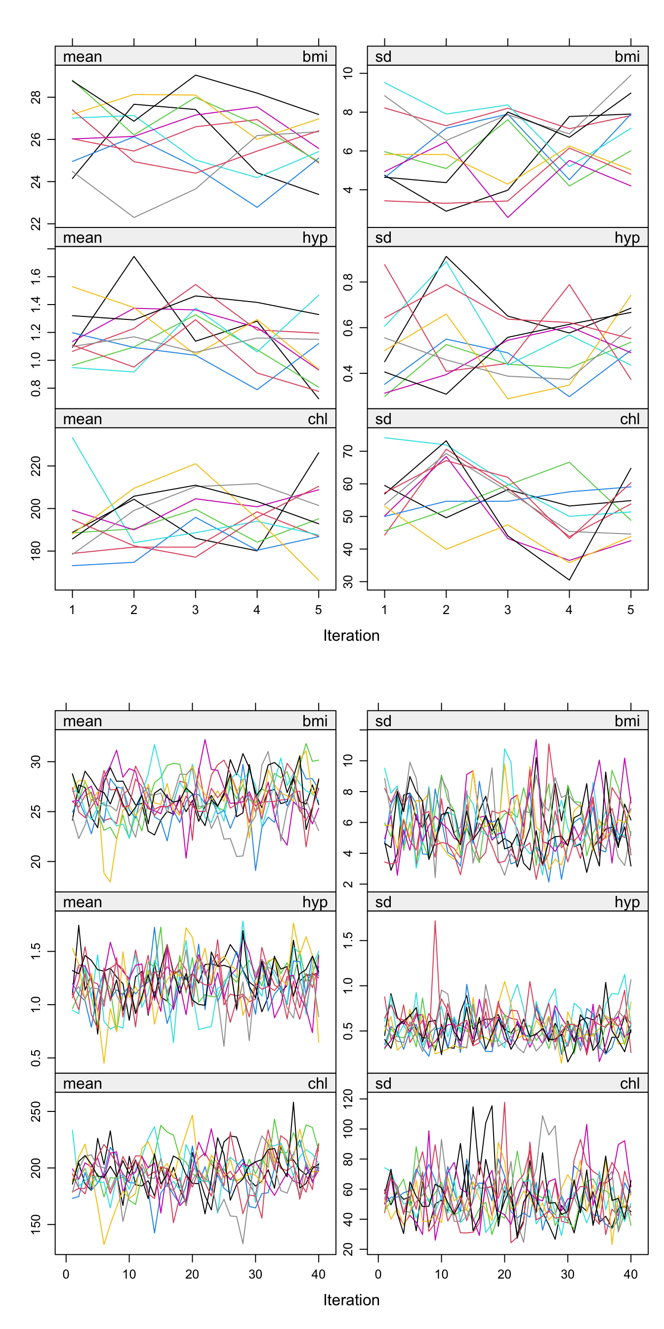
Figure 5.3: The mean and standard deviation of the three missing variables over the internal iterations of the MICE algorithm. The top panel shows the default 5 iterations for the 10 imputation datasets, and the bottom panel shows this after having been extended to 40 iterations.
We plotted our imputed datasets in Figure 5.2 to
explore the relationships between the variables. A further common
exploratory plot in multiple imputation would be to check that the
imputed values are plausible and could reasonably be believed to have
been values of possible observations. We can explore this with the
stripplot function, as shown in Figure 5.4. In such a
plot, we’re hoping to see that the imputed data in red is not so extreme
or unbelievable that we would not believe it could have been an observed
data point, and also whether there are trends being followed.
In Figure 5.4 we see some general
bunching of the imputations in areas where the observations have, such
as around 190 for chl, which is promising. We also see that there are
imputed values more extreme than we observed— we
would want to be careful to question whether these extremes are
plausible.
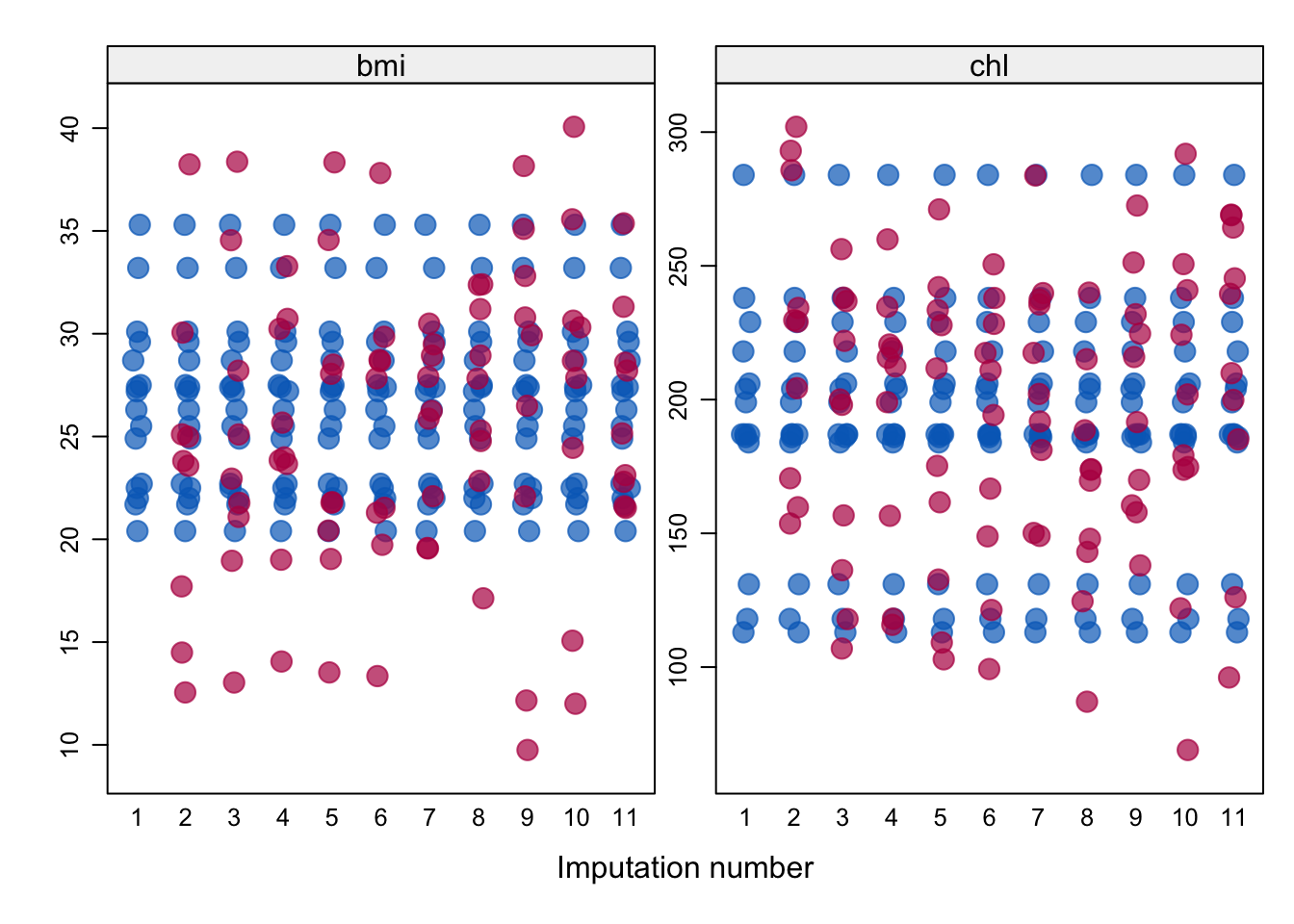
Figure 5.4: Strip plots of the imputed variables bmi and chl. The observed data is shown in blue, and imputed data in red. Imputation 1 is shown as the original, incomplete data, and the 10 imputations are shown proceeding this.
5.9.3 Imputation analysis
We now analyse each of each of
our imputed datasets. Recall that our aim was to estimate the parameters
\(\beta_0,\beta_\text{age},\beta_\text{chl},\beta_\text{age*chl},\sigma^2\)
for the regression model in Equation (5.3). We use the
function with() for this task:
nhanes_fit <- with(nhanes_imp, lm(bmi ~ chl * age))We produce an object of type mira, multiply imputed repeated
analyses, which contains the estimated regression parameters for each
of the 10 imputed datasets we created earlier. For instance, the summary
of the model fitted to the first imputed dataset is:
summary(nhanes_fit$analyses[[1]])##
## Call:
## lm(formula = bmi ~ chl * age)
##
## Residuals:
## Min 1Q Median 3Q Max
## -12.0483 -1.4156 0.2602 2.6360 4.7962
##
## Coefficients:
## Estimate Std. Error t value Pr(>|t|)
## (Intercept) 17.019780 8.040370 2.117 0.0464 *
## chl 0.088147 0.039157 2.251 0.0352 *
## age -4.792027 5.011114 -0.956 0.3498
## chl:age -0.003299 0.021579 -0.153 0.8799
## ---
## Signif. codes: 0 '***' 0.001 '**' 0.01 '*' 0.05 '.' 0.1 ' ' 1
##
## Residual standard error: 4.251 on 21 degrees of freedom
## Multiple R-squared: 0.5393, Adjusted R-squared: 0.4735
## F-statistic: 8.195 on 3 and 21 DF, p-value: 0.00084125.9.4 Analysis pooling
Finally, we pool our analyses together in step (3) of our multiple
imputation work-flow with the function pool():
(nhanes_pool <- pool(nhanes_fit))## Class: mipo m = 10
## term m estimate ubar b t dfcom
## 1 (Intercept) 10 18.644069364 5.256869e+01 5.114892e+01 1.088325e+02 21
## 2 chl 10 0.083297046 1.410073e-03 8.881682e-04 2.387058e-03 21
## 3 age 10 -3.631627438 2.066410e+01 2.845666e+01 5.196643e+01 21
## 4 chl:age 10 -0.006087487 4.483626e-04 3.977539e-04 8.858919e-04 21
## df riv lambda fmi
## 1 7.286312 1.0702913 0.5169762 0.6108920
## 2 9.384960 0.6928614 0.4092842 0.5046766
## 3 5.849503 1.5148169 0.6023567 0.6922247
## 4 7.707515 0.9758382 0.4938857 0.5884201We produce an object of type mipo, multiply imputed pooled object.
We can see the pooled estimates of our parameters of interest, which we
have referred to as \(\bar{\theta}\), via the estimate above. The
components of the variance of this are given, with the total being t,
and the proportion of the variance that is due to the missing data is
given by lambda. Note that although age is completely observed in
the data, this does not mean that this translates through into
estimating the coefficient \(\beta_\text{age}\) without missingness error,
because the bmi and chl were not fully observed.
We can explore the pooled estimate also with summary():
summary(nhanes_pool)## term estimate std.error statistic df p.value
## 1 (Intercept) 18.644069364 10.43228159 1.7871517 7.286312 0.1153885
## 2 chl 0.083297046 0.04885753 1.7048969 9.384960 0.1210228
## 3 age -3.631627438 7.20877448 -0.5037788 5.849503 0.6328217
## 4 chl:age -0.006087487 0.02976394 -0.2045256 7.707515 0.8432399This suggests from the pooled p-value estimates that the age and
chl*age terms are not required in our model.