Chapter 8 Variational inference
\(\def \mb{\mathbb}\) \(\def \E{\mb{E}}\) \(\def \P{\mb{P}}\) \(\DeclareMathOperator{\var}{Var}\) \(\DeclareMathOperator{\cov}{Cov}\)
| Aims of this section |
|---|
| 1. Appreciate the limitations of inference via sampling schemes, and that approximate inference can be a useful alternative in some situations. |
| 2. Understand the need to assess ‘agreement’ between distributions as part of this approximation process, and the role that KL divergence and ELBO play in this. |
| 3. Have an awareness of how approximate inference is practically implemented, including the choice of approximation using the mean field family and the optimisation process using coordinate ascent. |
In this chapter we are going to introduce variational inference: an approach to approximating probability distributions that can be used in Bayesian inference, as an alternative to MCMC. Variational methods are popular for implementing Bayesian approaches in machine learning, and work well with large and complex data sets.
This and the following chapter are based on a review article (Blei, Kucukelbir, and McAuliffe 2017).
8.1 Background theory
8.1.1 Jensen’s inequality
Although not necessary for understanding the concepts in this chapter, they hinge on this important result. Jensen’s inequality relates to the integrals of convex functions, and we are interested in this applied to expectations of logarithms (because \(\log\) is a concave function): \[\log ( \E (f(x)))\geq \E(\log(f(x))),\] for \(f(x)>0\).
8.1.2 Kullback-Leibler Divergence
The Kullback-Leibler (KL) divergence is a measure of how one probability distribution is different from a second. Often we might compare distributions, such as two choices of prior distribution, by looking at summaries such as moments (mean/variance) or quantiles. However, these can only give snapshots of the similarity between two distributions. The KL divergence is a summary that takes into account the entire functional form of the distributions across all real values.
We will define KL divergence only in terms of continuous distributions, but note that this can similarly be defined for discrete distributions. The KL divergence between the distribution \(p\) and \(q\) is given by \[\begin{align} KL(p \ || \ q) &= \int_{\mathbb{R}} p(x) \log \left( \frac{p(x)}{q(x)} \right) dx \\ &= \E_{p(x)} \left[ \log \left( \frac{p(x)}{q(x)} \right) \right] \\ &= \E_{p(x)} \left[ \log p(x) \right] - \E_{p(x)} \left[\log q(x) \right]. \end{align}\] Note the the KL divergence is defined only if \(q(x)=0\) implies that \(p(x)=0\), for all \(x\), and the contribution of such to the KL measure is interpreted as 0.
Important properties of the KL divergence include:
- Non-symmetry, i.e. \(KL(p \ || \ q) \neq KL(q \ || \ p)\).
- Non-negative, i.e. \(KL(p \ || \ q) \geq 0\) for all \(p,q\). Note that this result is proven based on Jensen’s inequality.
- Equality identifying, i.e. \(KL(p \ || \ q)=0\) if and only if \(p(x)=q(x)\) for all \(x\).
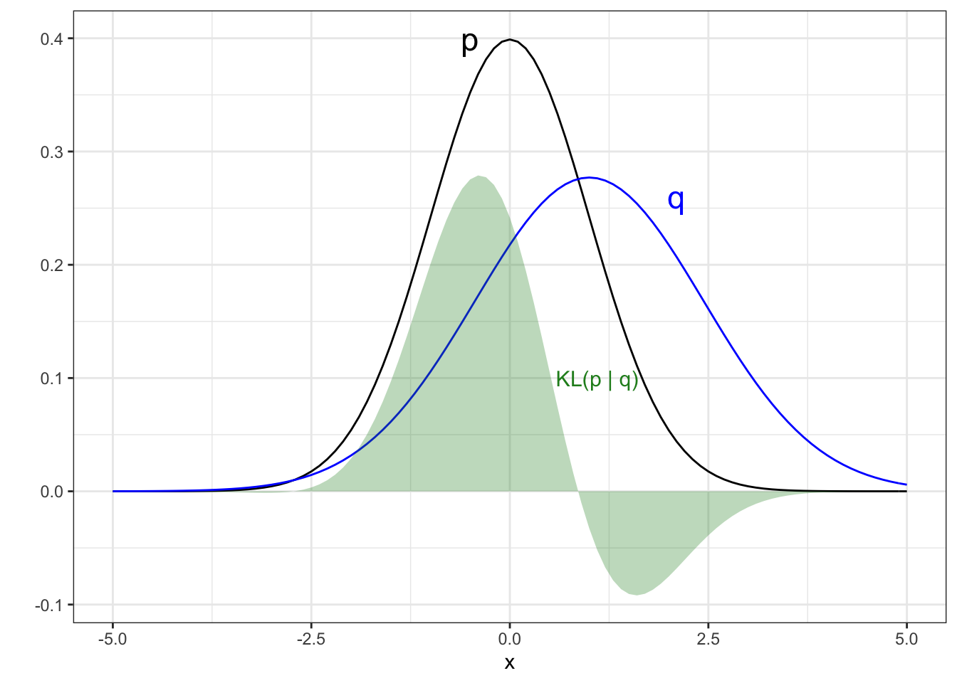
Figure 8.1: Example of the KL divergence between two Gaussian distributions. The contribution to the KL divergence is shown by the green region, with the KL figure being the area of this region.
The KL divergence is depicted in Figure 8.1, showing the densities of two Gaussian distributions, \(p\) (black) and \(q\) (blue). The contribution to the KL divergence, \(KL(p \ || \ q)\), is shown by the green region, and the actual value of the KL divergence is the area of this region. We see that the disagreement between distributions is not handled uniformly by the KL divergence. In this example the contribution to the KL divergence of \(p\) from \(q\) is not symmetric, it has higher penalty for \(p\) having density where \(q\) has little and less penalty for not having significant density where \(q\) has high density. We will return to this behaviour of the KL divergence later, as it plays an important role as to the use of \(KL(p \ || \ q)\) versus \(KL(q \ || \ p)\), which will produce different values. In this example, \(KL(p \ || \ q)=0.42\) and \(KL(q \ || \ p) = 0.51\).
8.1.3 Optimisation with coordinate ascent
Coordinate ascent is an optimisation procedure to find \[\underset{\mathbf{x}\in \mathbb{R}^n}{\arg\max} \ f(\mathbf{x}).\] The main idea is to find the maximum of \(f(\cdot)\) by maximising along one dimension at a time, holding all other dimensions constant—it being much easier to deal with one-dimensional problems. We therefore loop through each dimension \(i \in 1,\ldots,n\) over a number of steps \(k\), setting \[x_i^{k+1} = \underset{y \in \mathbb{R}}{\arg\max} \ f(x_1^{k},\ldots, x_{i-1}^k,y,x_{i+1}^k,\ldots,x_n^k).\] An optimal update scheme involves using the gradient of the above function and setting \[x_i^{k+1} = x_i^{k} + \epsilon \frac{\partial f(\mathbf{x})}{\partial x_i},\] for \(i=1,\ldots,n\). Usually, a threshold will be set to monitor that convergence has been met, stopping the coordinate ascent algorithm once the difference between \(x_i^{k+1}\) and \(x_i^k\) is under such threshold.
We will not concern ourselves with the details of why this works, but it is enough to know the algorithm and that we end up moving in one dimension at a time, iteratively climbing the function to the maximum. We will be using this approach in the next chapter.
8.1.4 Stochastic optimisation
Another option for optimisation that we will look at in this part is stochastic optimisation. Here, the idea is to introduce \(h^k(\mathbf{x})\sim H(\mathbf{x})\), where \(\E\left[h^k(\mathbf{x})\right]=\frac{df(\mathbf{x})}{d\mathbf{x}}\). Similarly to the above we update in each dimension with \[x_i^{k+1} = x_i^k + \epsilon^k h^k(x_i^k),\] where there are some conditions that we will not cover on the choice of \(\epsilon\). Again, we won’t concern ourselves too much with the underlying theory here—but will show you this implementation in practice at the end of this part of the course.
8.2 Motivation for approximate inference approaches
8.2.1 Intractable integrals
When we implement Bayesian inference, our goal is evaluate the posterior distribution \[p(\theta | x)= \frac{p(\theta)p(x|\theta)}{p(x)} = \frac{p(x, \theta)}{p(x)},\] to learn about some parameters of interest \(\theta\), given observations \(x\). For conciseness, we will write \(p(x,\theta)\) instead of \(p(\theta)p(x|\theta)\), but you should be thinking of multiplying a prior \(p(\theta)\) and a likelihood \(p(x|\theta)\) any time you see the joint density \(p(x,\theta)\).
The numerator in the above is often tractable and easily evaluated. The difficulty in evaluating the posterior arises from the denominator, which we often refer to as the normalising constant and is also often called the evidence. This is given by \[p(x)=\int_\Theta p(x, \theta) d \theta.\]
Previously, we used MCMC to get around this problem, as it was only necessary to be able to evaluate \(p(x, \theta)\) and not \(p(x)\). As we will see shortly, variational inference has the same feature.
8.2.2 Variational approach to intractable integrals
Variational inference is an approximation to the posterior. Unlike MCMC, the main computational effort is in constructing the approximation. We approximate \(p(\theta|x)\) by an alternative distribution, \(q^*(\theta)\). This distribution will be simple enough to be tractable, so that we can evaluate quantities of interest such as \(\E_{q^*}(\theta)\) directly, or obtain i.i.d. samples very easily.
The aim of variational inference therefore is to find the particular form of \(q^*(\cdot)\) so that it is both tractable, and it is a good approximation to \(p(\theta|x)\), which is intractable. We will assume that we have a family of candidate distributions, which we refer to as \(\mathcal{Q}\). We will return to exactly what form this family will take later, but for now you can imagine that \(\theta\) is one-dimensional, and \(\mathcal{Q}\) could be the family of all Gaussian distributions. The process of variational inference in such a scenario would be choosing the value of the mean and variance of the Gaussian distribution that is most similar to the posterior we are interested in.
The benefit of variational inference is that it tends to be very fast, and this is the reason for its choice over MCMC. Note that this is a trade-off situation: you are trading having a solution quickly in exchange for it no longer being the exact posterior. The speed makes it more appealing in problems involving large data sets. Note that it is generally the case that variational inference underestimates the variance of the posterior, and so it is better suited for problems where this uncertainty estimate is not the primary interest.
In the next sections we will cover the details of variational inference, which is ultimately the process of choosing which \(q(\theta) \in \mathcal{Q}\) is the ‘best’ approximation to \(p(\theta|x)\). Note here that although we write \(q(\theta)\), this is a simplification. There will be some parameters involved in this distributional definition—the one-dimensional Gaussian example would involve there being a choice of the value of the mean and variance of such a Gaussian, and these would be the variational parameters. We do not include these in our notation to allow flexibility in the form of the distributions in the family \(\mathcal{Q}\). Further, the values that these variational parameters will take will depend on the observed data \(x\) in some way. We could therefore write \(q(\theta | \phi,x)\) to explicitly state this, where \(\phi\) are the variational parameters. However, for readability throughout the following we will drop this and only use \(q(\theta)\).
8.3 Approximate inference as an optimisation problem
We have stated that variational inference involves approximating the posterior of interest, \(p(\theta|x)\), with a tractable distribution \(q^*(\theta)\). This approximate distribution, \(q^*(\theta)\), is chosen as the ‘best’ candidate from a family of distributions \(q(\theta)\in \mathcal{Q}\). In this context, by ‘best’ candidate, we mean the distribution in \(\mathcal{Q}\) that is most similar in functional form to the posterior. We will use the Kullback-Leibler divergence to quantitatively measure the ‘similarity’ between the candidate distributions and the posterior of interest. To formalise the choice of the approximate distribution, this is \[\begin{equation} q^*(\theta) = \underset{q(\theta)\in \mathcal{Q}}{\arg\min} \ KL(q(\theta) \ || \ p(\theta|x)). \end{equation}\] || p(|x)). \end{equation}
So, our inference approach would be to calculate the KL divergence from \(p(\theta|x)\) for each \(q(\theta)\in \mathcal{Q}\) and then choosing the distribution with the smallest divergence. We’ll now examine how we deal with the unknown normalising constant \(p(x)\). First note that \[\begin{align} KL(q(\theta) \ || \ p(\theta|x)) &= \E_q\left[ \log q(\theta) \right] - \E_q \left[ \log p(\theta|x) \right] \\ &= \E_q\left[ \log q(\theta) \right] - \E_q \left[ \log \left( \frac{p(x,\theta)}{p(x)} \right) \right] \\ &= \E_q\left[ \log q(\theta) \right] - \E_q \left[ \log p(x,\theta) \right] + \E_q \left[ \log p(x) \right] \\ &= \E_q\left[ \log q(\theta) \right] - \E_q \left[ \log p(x,\theta) \right] + \log p(x). \end{align}\] Where we obtain the final line in the above because \(p(x)\) is a constant with respect to \(q\), so \(E_q(\log p(x))=\log p(x)\). So our issue is that we cannot actually calculate the KL divergence for each \(q(\theta)\in \mathcal{Q}\), because we cannot evaluate the final term in the above involving \(p(x)\).
We define another measure, which is an element of the KL divergence calculation: \[KL(q(\theta) \ || \ p(\theta|x)) = \underbrace{\E_q\left[ \log q(\theta) \right] - \E_q \left[ \log p(x,\theta) \right]}_{-ELBO(q)} + \log p(x).\] This is the evidence lower bound, or variational lower bound, given by \[\begin{align} ELBO(q) &= \E_q \left[ \log p(x,\theta) \right] - \E_q\left[ \log q(\theta) \right] \\ &= \E_q \left[ \log \left ( \frac{p(x,\theta)}{q(\theta)} \right) \right]. \end{align}\] Again, we are simplifying things somewhat by referring to ELBO as being a function of \(q\) alone, but we do this to highlight that \(q(\theta) \in \mathcal{Q}\) will be the only varying input to the ELBO in practice (as our \(x\) have been observed). Therefore \[KL(q(\theta) \ || \ p(\theta|x)) = \log p(x) - ELBO(q).\] The good news is that \(ELBO(q)\) is something that we can calculate, as we are assuming that \(p(x,\theta)\) is tractable. If the approach of variational inference was to choose the \(q(\theta) \in \mathcal{Q}\) which minimises \(KL(q(\theta) \ || \ p(\theta|x))\), then because \(\log p(x)\) is constant with respect to \(q\), this is equivalent to maximising \(ELBO(q)\).
Variational inference therefore approximates \(p(\theta|x)\) with \[\begin{equation} q^*(\theta) = \underset{q(\theta)\in \mathcal{Q}}{\arg\max} \ ELBO(q(\theta)). \end{equation}\]). \end{equation} The inference approach is an optimisation problem because once we have a chosen family of candidate distributions, \(\mathcal{Q}\), we merely need to find the optimal candidate for the ELBO.
8.3.1 Exploring the ELBO
We have seen that variational inference is all about finding a distribution function that maximises the ELBO. Let us explore this further to gain an understanding of what this means for our chosen approximation to the posterior. We manipulate the above expression for the ELBO: \[\begin{align} ELBO(q) &= \E_q \left[ \log \left ( \frac{p(x,\theta)}{q(\theta)} \right) \right] \\ &= \E_q \left[ \log \left ( \frac{p(\theta)p(x|\theta)}{q(\theta)} \right) \right] \\ &= \E_q \left[ \log p(x|\theta) \right] + \E_q \left[ \log \left ( \frac{p(\theta)}{q(\theta)} \right) \right] \\ &= \E_q \left[ \log p(x|\theta) \right] - \E_q \left[ \log \left ( \frac{q(\theta)}{p(\theta)} \right) \right] \\ &= \E_q \left[ \log p(x|\theta) \right] - KL(q(\theta) \ || \ p(\theta)). \end{align}\] By choosing the \(q\) that maximising this expression:
- \(\E_q \left[ \log p(x|\theta) \right]\) is the expectation with respect to \(q\) of the likelihood of the data. Maximising this means finding the function \(q\) that explains the data.
- \(KL(q(\theta) \ || \ p(\theta))\) is the divergence from the prior. Minimising this (because of the minus sign in the ELBO expression above) means finding the function \(q\) that is similar to the prior. So intuitively, maximising the ELBO makes sense as we have the delicate balance that we would expect between remaining similar to our prior distribution, whilst matching the observed data.
We perform inference by finding the \(q\) that maximises the ELBO, but the value of the ELBO for this function can also be a useful measure in itself. Recall from above that \[KL(q(\theta) \ || \ p(\theta|x)) = \log p(x) - ELBO(q),\] and also that \(KL(\cdot || \cdot) \geq 0\). Therefore \[ELBO(q) \leq \log p(x),\] with equality if and only if \(q(\theta)=p(\theta|x)\). This expression is where ELBO gets its name—it is the lower bound of the evidence (we said at the start of this chapter that a common name for the normalising constant is the evidence). Because of this relation, \(ELBO(q^*)\) has been used as a model selection tool, under the assumption that equality has almost been reached. We won’t discuss this further, as there is no justification from theory that this is the case.
8.3.2 Forward and reverse variational inference
We defined the variational approach as approximating the posterior with the distribution \[q^*(\theta) = \underset{q(\theta)\in \mathcal{Q}}{\arg\min} \ KL(q(\theta) \ || \ p(\theta|x)),\] so that we choose the distribution from the candidate family with smallest KL divergence from the posterior. You might have questioned whether this is the only choice. Recall that the KL divergence is not symmetric so that \[KL(q(\theta) \ || \ p(\theta|x)) \neq KL(p(\theta|x) \ || \ q(\theta)),\] and so it’s not immediately obvious why we have made the decision to use the KL divergence that we have done. Our decision of using \(KL(q(\theta) \ || \ p(\theta|x))\) is known as reverse KL, and the alternative option of using \(KL(p(\theta|x) \ || \ q(\theta))\) is known as forward KL. Here we will discuss briefly how inference is affected by the two approaches.
8.3.2.1 Forward KL
In forward KL we find the \(q\) that minimises \[KL(p(\theta|x) \ || \ q(\theta))=\int p(\theta|x) \log \left( \frac{p(\theta|x)}{q(\theta)} \right)d\theta,\] and this ordering is referred to as weighting the difference between \(p(\theta|x)\) and \(q(\theta)\) by \(p(\theta|x)\).
Consider the values of \(\theta\) such that \(p(\theta|x)=0\). In the above, it does not matter what the value of \(q(\theta)\) is in terms of the contribution to the KL divergence. So there is no consequence for there being large disagreement between the two functions at these values of \(\theta\). Minimising the forward KL divergence therefore optimises \(q\) to be non-zero wherever \(p(\theta|x)\) is non-zero, and penalises most heavily at the values of \(\theta\) with high density in \(p(\theta|x)\). This leads to a good global fit, and this approach being known as moment matching (because the mean of the posterior is mimicked with highest importance) or zero avoiding (because we are avoiding \(q(\theta)=0\) when \(p(\theta|x)>0\)).
To see the outcome of this approach visually, we show a one-dimensional posterior in Figure 8.2 that has two modes. If the candidate distribution family was Gaussian, then two possibilities for the approximate distribution are shown in the two panels, with the optimal choice under forward KL divergence being the right hand panel. You can see from the contribution to the KL divergence in green that not placing density where there is density in the posterior is highly penalised by the forward KL, which forces the optimal choice to be the right have option, even though the approximate distribution has its mode in a region of very low density in the posterior.
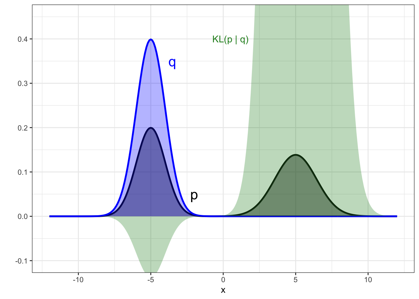
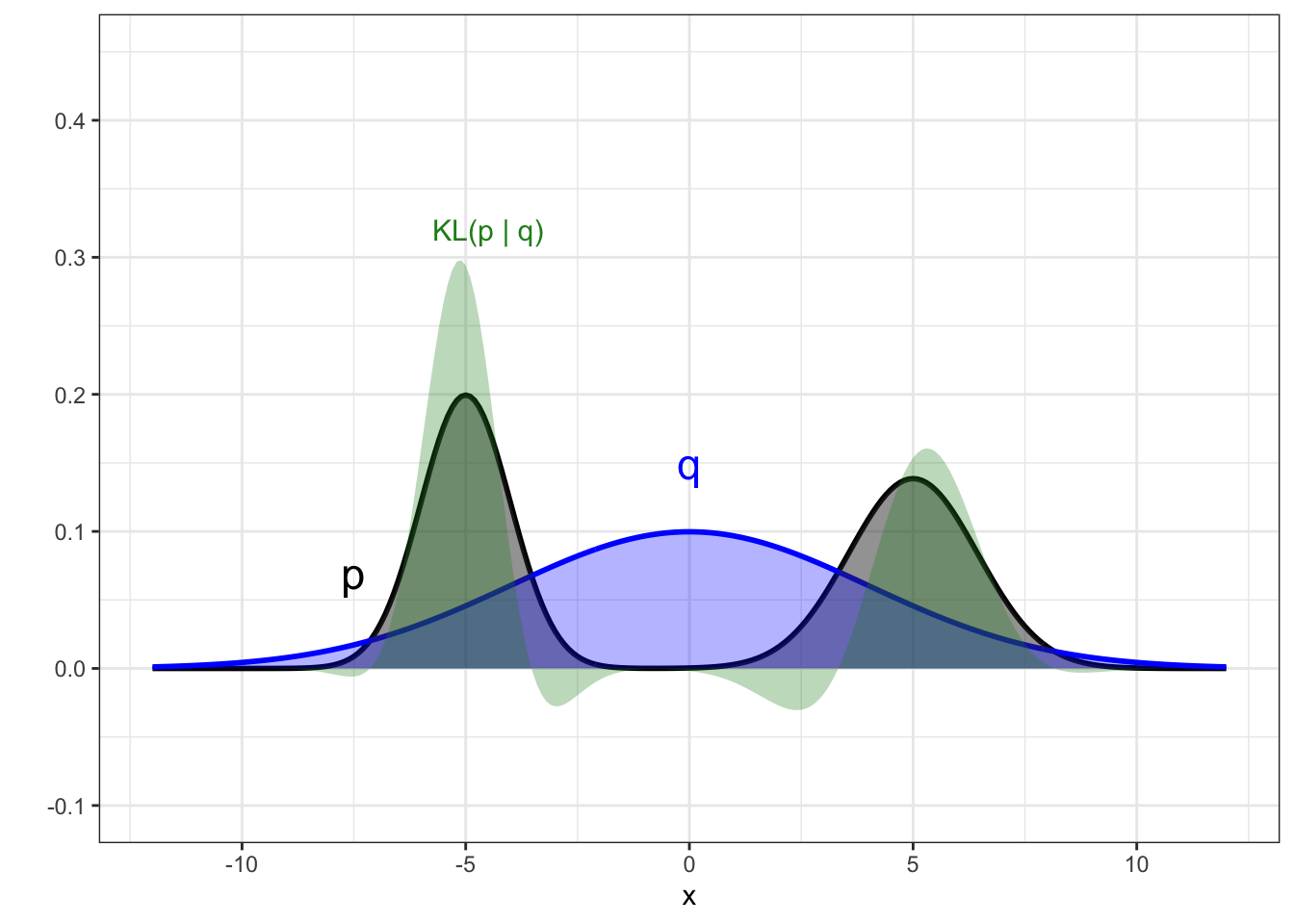
Figure 8.2: Example of the forward KL divergence when the target posterior is multi-modal. Target posterior is shown in black, and the two panels show two alternative candidate distributions from a Gaussian family (blue). The contribution to the KL divergence is shown by the green region, with the KL figure itself being the area of this region.
8.3.2.2 Reverse KL
In reverse KL (the version that is most commonly used in practice and that we have introduced as our approach for variational inference) we find the \(q\) that minimises \[KL(q(\theta) \ || \ p(\theta|x))=\int q(\theta) \log \left( \frac{q(\theta)}{p(\theta|x)} \right)d\theta,\] and so now \(q(\theta)\) is the ‘weight’.
In this scenario, values of \(\theta\) that lead to \(q(\theta)=0\) have no penalty. So there is no penalty for ignoring the region where the posterior has density. Instead, it is the region where \(q(\theta)>0\) that contributes large penalties to the KL divergence. Therefore, it does not matter if \(q(\theta)\) fails to place density on areas of the posterior that have density, as long as the region where we do place density very closely mimics the posterior. The optimal approximation will avoid spreading density widely and will have good local fits to the posterior. This approach is known as mode seeking (because the mode of the posterior is mimicked with highest importance) or zero forcing (because we are often forced to allow \(q(\theta)=0\) in some areas even if the posterior is not).
To see the outcome of this approach visually, we show the same scenario as Figure 8.2 for the reverse KL in Figure 8.3. Now the optimal choice under has switched and is the distribution on the left. You can see from the contribution to the KL divergence in green that not placing density where there is density in the posterior is not penalised at all in reverse KL (the right mode is ignored by the approximate distribution in the left panel), but that matching is highly penalised where we do choose to put density.
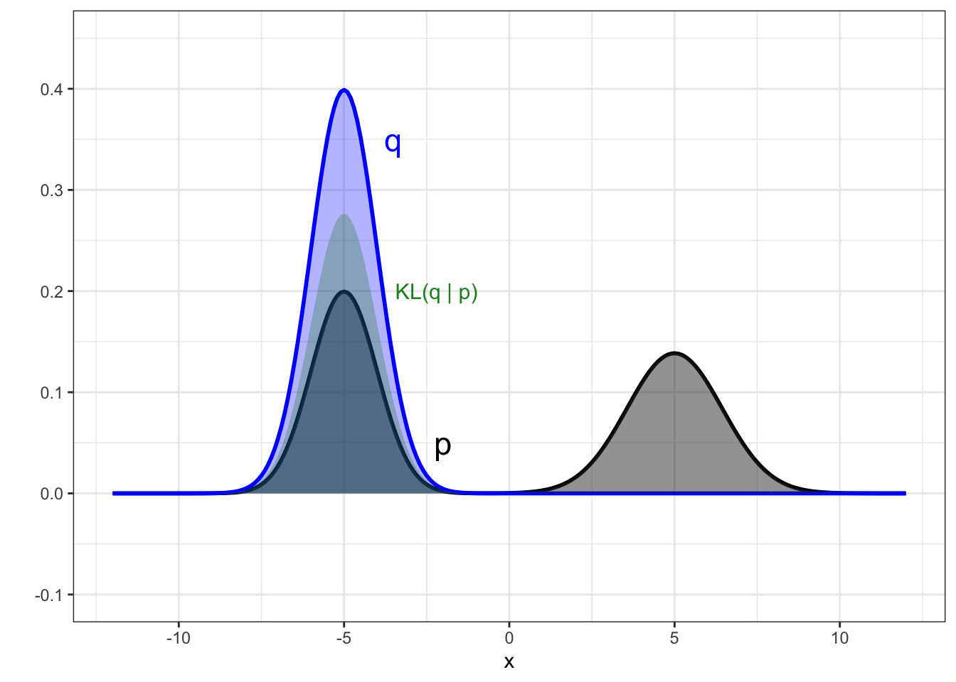
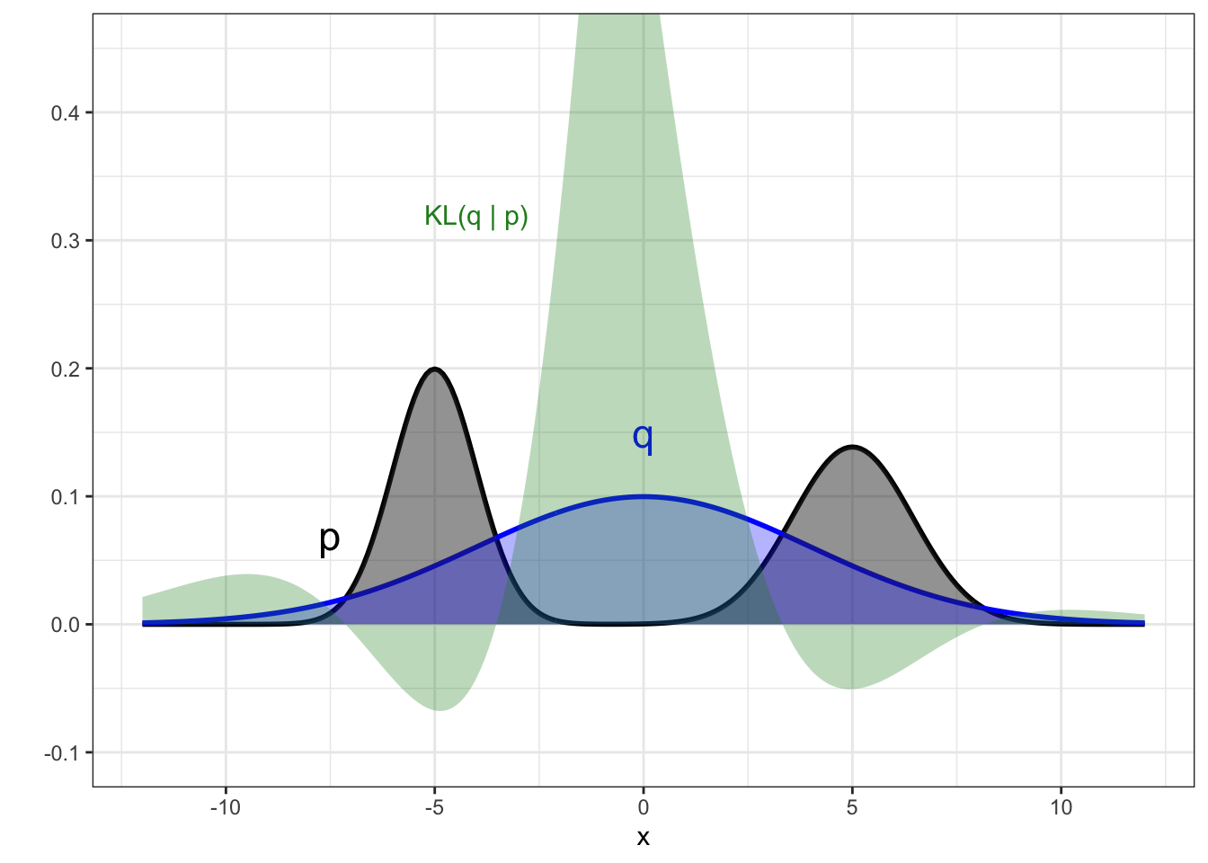
Figure 8.3: Example of the reverse KL divergence when the target posterior is multi-modal. Target posterior is shown in black, and the two panels show two alternative candidate distributions from a Gaussian family (blue). The contribution to the KL divergence is shown by the green region, with the KL figure itself being the area of this region.
8.4 The variational family of distributions
We have now seen the main concept of variational inference. This involves specifying a family of candidate distributions from which we will choose our approximate distribution from, referred to as \(\mathcal{Q}\) in the above. In practice, a decision needs to be made about this. The family of distributions needs to be flexible enough that we believe it will contain distributions able to closely mimic our true posterior, whilst being simple enough that we can calculate the ELBO and maximise it.
8.4.1 Mean-field family
Here we will discuss the current most popular choice in practice, known as the mean-field variational family. For a general distribution \(q(\theta)\in\mathcal{Q}\), we assume that the dimensions of \(\theta\) are mutually independent and therefore the density of a general distribution can be simplified as \[q(\theta) = \prod_{i=1}^m q_i(\theta_i),\] where \(\theta=(\theta_1,\ldots,\theta_m)\). Each \(q_i(\cdot)\) can be specified as generally as needed, dependent upon the parameter it is describing, i.e. we might have a two-dimensional parameter set and assume that \(q_1\) comes from the family of Gaussians and \(q_2\) comes from the family of gammas.
8.4.2 Correlation cannot be replicated
The mean-field family cannot capture correlations between parameters because our family of candidate distributions are defined to have independent components. As an example, see Figure 8.4, which shows a two-dimensional true posterior in blue with high correlation. The best approximation from a mean-field family will take the form of that in green. As the name of the family suggests, the approximation picks out moments of the underlying distribution, so that the estimate of the mean in both dimensions will be a good approximation to the true posterior.
The correlation cannot be replicated as the candidate family enforces independence. Further, note that the consequence of this is that the variance in the marginals is under-estimated significantly—this was noted at the start of this chapter that variational inference commonly suffers from this problem and this is main reason for this.
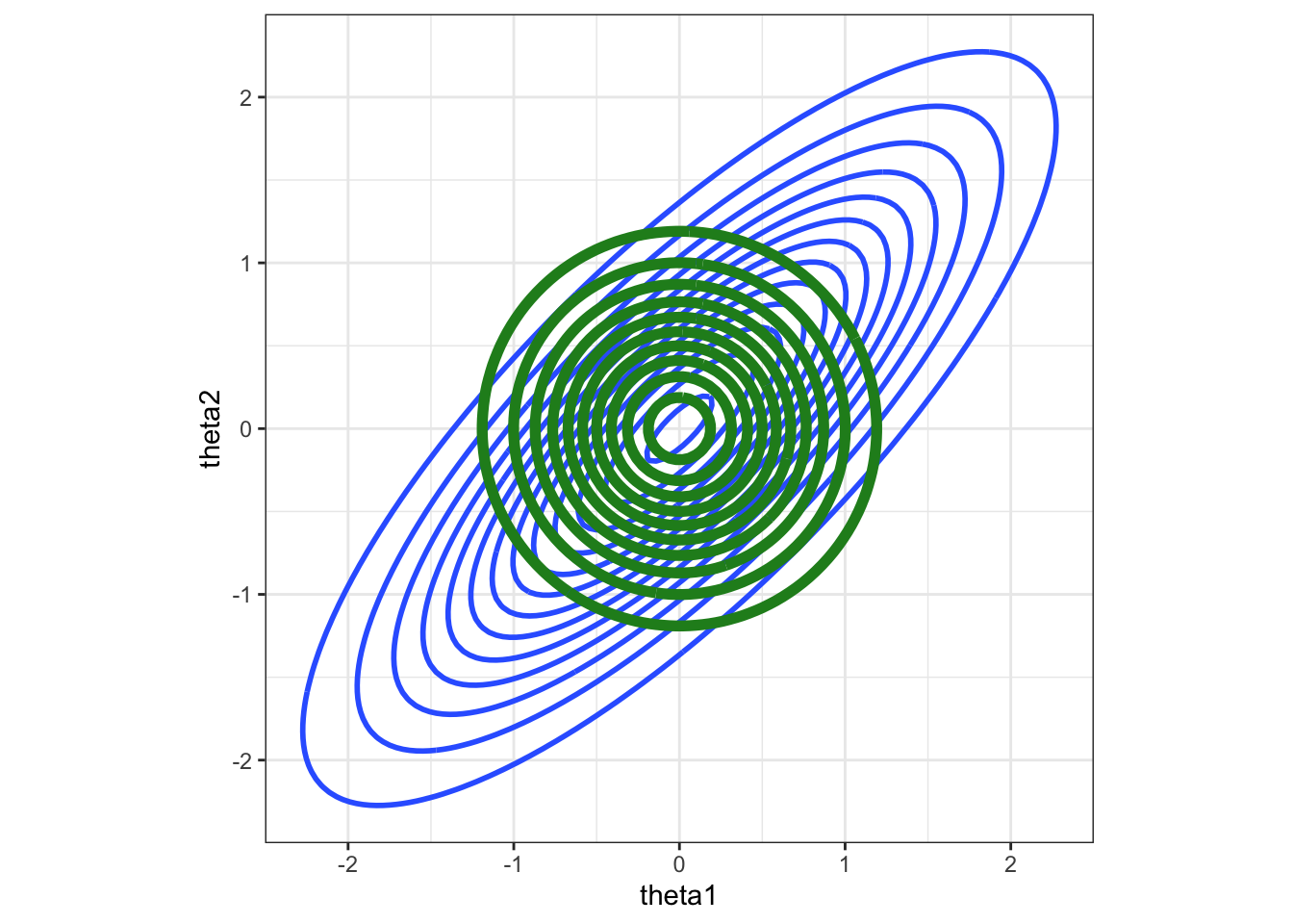
Figure 8.4: Example of how correlations between parameters are handled using a mean-field approximation in variational inference. Here we have a two-dimensional parameter set, and if the true distribution was highly correlated (blue), this cannot be captured by the optimal mean-field approximation (green).
8.4.3 Why mean-field is useful
So if the mean-field family means we cannot reproduce correlations between parameters, why is it used? Variational inference involves us being able to maximise the ELBO and finding the \(q\in\mathcal{Q}\) which does this. Recall that the ELBO is an expectation, so that \[ELBO(q) = \E_q \left[ \log \left ( \frac{p(x,\theta)}{q(\theta)} \right) \right] = \int_\Theta q(\theta) \log \left ( \frac{p(x,\theta)}{q(\theta)} \right) d\theta.\] If \(\theta\) is multi-dimensional, so that \(\theta = (\theta_1,\ldots,\theta_m)\) then this integral is explicitly \[\int_{\Theta_1} \ldots \int_{\Theta_m} q(\theta_1,\ldots,\theta_m) \log \left ( \frac{p(x,\theta_1,\ldots,\theta_m)}{q(\theta_1,\ldots,\theta_m)} \right) d\theta_1\ldots d\theta_m,\] which is going to very easily enter the realm of being intractable, which is what we need to avoid here! This is the reason that the mean-field approximation is commonly used in practice, the independence between dimensions means that this integral can be simplified significantly into a product of integrals.
Remember: variational inference is a trade-off where we are having to make simplifications (and thus loss of precision) in exchange for speed.