Chapter 7 Cross-validation
\(\def \mb{\mathbb}\) \(\def \E{\mb{E}}\) \(\def \P{\mb{P}}\) \(\DeclareMathOperator{\var}{Var}\) \(\DeclareMathOperator{\cov}{Cov}\)
| Aims of this chapter |
|---|
| 1. Understand cross-validation as a tool for both testing the predictive ability of a model, and for parameter estimation. |
| 2. Learn about computational short-cuts for implementing cross-validation. |
| 3. Explore the link between cross-validation and AIC for model selection. |
We consider problems where the main interest is in prediction rather than inference: predicting the value of some dependent variable \(y\) given independent variables \(x\). We suppose we have a data set \[D=\{(x_i, y_i),\, i=1,\ldots,n\},\] and we want to test the performance of some model or algorithm that, using these data, will predict \(y\) for any value of \(x\).
The usual practice is to divide the data \(D\) into a training set and a test set. For each \(x\) in the test set, we would predict the corresponding \(y\), using the training data only. For small data sets, this division may not be desirable; we may need to use all the data just to get good predictions and/or to reduce the uncertainty in our predictions as much as possible.
When we have a small data set, we can assess the performance of our model using cross-validation instead. The basic idea is as follows.
For \(i=1,\ldots,n\) we
- obtain a reduced data set \(D_{-i}\) by removing the observation \((x_i,y_i)\) from the full data set \(D\);
- re-fit the model using the reduced data set \(D_{-i}\), and predict the observation we removed in step 1: we obtain a prediction \(\hat{y}_i\) of the dependent variable given \(x_i\).
In removing any single observation, we’re hoping that the fitted model using the data \(D_{-i}\) is similar to the fitted model based on all the data \(D\); predictions wouldn’t change much ‘in general’. We then get a sample of \(n\) predictions errors \(\hat{y}_1 - y_1,\ldots,\hat{y}_n - y_n\) with which we can evaluate our model.
What we calculate precisely in step (2), and what we do with the results, will depend on the problem. We’ll give two examples in this chapter. Note that this procedure is sometimes referred to as leave-one-out cross-validation, as we are leaving out a single observation in turn. \(k\)-fold cross-validation refers to leaving out \(k\) observations at a time. We will not consider this here, but the concept is the same.
7.1 Cross-validation in classification
7.1.1 The Palmer penguins data
We consider a data set from Gorman et al. (2014) and provided in an R package palmerpenguins (Horst, Hill, and Gorman 2020). In this example, we suppose the aim is to predict (“classify”) the species of a penguin (one of Adelie, Chinstrap and Gentoo) based on the measurements of bill length, bill depth and flipper length. One can imagine that it may be difficult to obtain a large data set for this sort of problem.

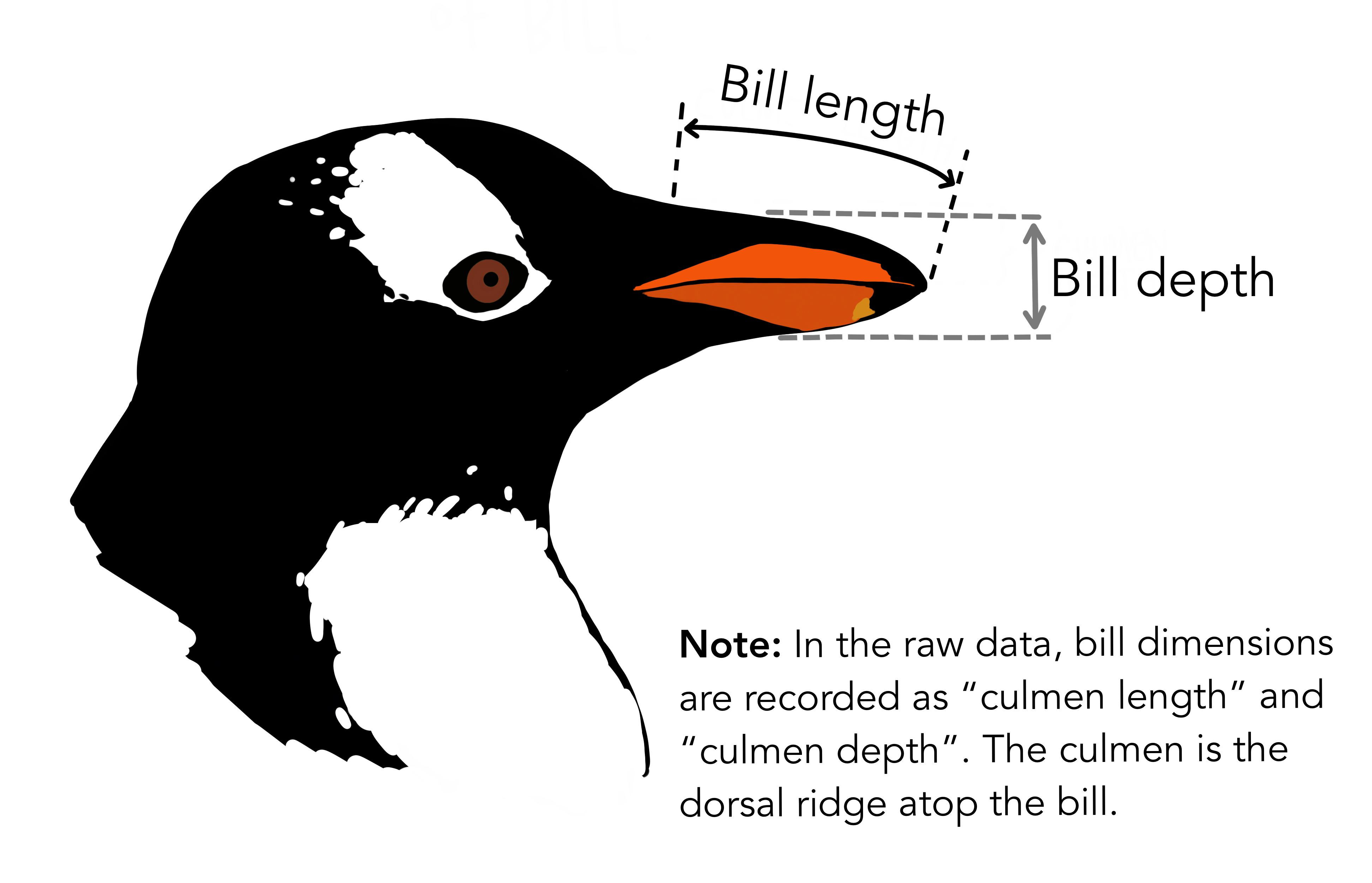
Figure 7.1: Introducing the Palmer penguins. Artwork by Allison Horst.
The data look like this:
## # A tibble: 6 × 4
##   species bill_length_mm bill_depth_mm flipper_length_mm
##   <fct>            <dbl>         <dbl>             <int>
## 1 Adelie            39.1          18.7               181
## 2 Adelie            39.5          17.4               186
## 3 Adelie            40.3          18                 195
## 4 Adelie            NA            NA                  NA
## 5 Adelie            36.7          19.3               193
## 6 Adelie            39.3          20.6               190
There are 333 complete observations, so we have a data set \(D=\{(y_i, x_i),\,i=1,\ldots,333\}\), where, for the \(i^\text{th}\) penguin:
- \(y_i = 1\), \(2\) or \(3\) if the species is Adelie, Chinstrap or Gentoo, respectively, and
- \(\mathbf{x}_i\) is a vector of the three measurements: bill length, bill depth and flipper length (all in mm).
For a new penguin with measurements \(\mathbf{x}^*\), the aim would be to classify the species (\(y^*\)) given this measurement information alone.
Note that the penguin data from the palmerpenguins package contains 344 penguins, however only 333 of these have complete observations for the three measurement variables and the species type. We will not be considering this incomplete information in our analysis here, so have removed these individuals from the data we work with.
7.1.2 The \(K\)-nearest neighbours algorithm (KNN)
KNN is a simple algorithm for classification. There is no actual model, and just one parameter, \(K\), to choose. Given a new penguin with measurements \(\mathbf{x}\), the species is classified as follows:
- For the penguins \(i=1,\ldots,333\) in our data set \(D\), calculate the Euclidean distance \(||\mathbf{x}_i - \mathbf{x}||\).
- Find the \(K\) smallest Euclidean distances. This means that we have identified the \(K\) penguins in the data set \(D\) with measurements closest to the measurements \(\mathbf{x}\) of the new penguin. These are the \(K\) nearest neighbours.
- Classify the species of the new penguin as the species that occurred the most out of the \(K\) penguins found in step (2). If there is a tie, pick a species at random from those tied.
7.1.3 Implementing cross-validation in KNN
We can implement the KNN algorithm, using our training set of 333 penguins, for any measurement information that is obtained for a new penguin. However, we have no understanding of how well this algorithm is working, i.e. its prediction ability. We can asses how well this algorithm is working using cross-validation. We do the following, for \(i=1,\ldots,333\):
- Remove penguin \(i\) from the data set \(D\), to obtain a reduced data set \(D_{-i}\).
- Calculate the Euclidean distances \(||\mathbf{x}_j -\mathbf{x}_i||\) for each \(\mathbf{x}_j\) in the reduced data set \(D_{-i}\). This would involve \(j=1,\ldots, i-1,i+1, \ldots, 333\).
- Find the \(K\) penguins in \(D_{-i}\) with the smallest Euclidean distances from step (2), and obtain their species.
- Obtain the predicted species \(\hat{y}_i\) of the \(i\)-th penguin as the species that occurred the most in step (3).
We do this in R in the following. As we’re using Euclidean distances, we’ll convert the independent variables to be on (roughly) the same scale. If we did not do this, our algorithm could be placing more weight on classifying the penguins based on only one of the three measurements. To see this, we note the summary information of the three variables in Table 7.1. The scale of the flipper length variable is much larger than that of the bill depth, and therefore the distance measurement used as part of the KNN algorithm will be dominated by the differences in flipper length, causing this to be the determining variable for the classification process. When we scale the measurements we get comparable variables, as shown in Table 7.2.
| Bill length | Bill depth | Flipper length | |
|---|---|---|---|
| Min. :32.10 | Min. :13.10 | Min. :172 | |
| Median :44.50 | Median :17.30 | Median :197 | |
| 3rd Qu.:48.60 | 3rd Qu.:18.70 | 3rd Qu.:213 |
| Bill length (scaled) | Bill depth (scaled) | Flipper length (scaled) | |
|---|---|---|---|
| Min. :-2.17471 | Min. :-2.06418 | Min. :-2.0667 | |
| Median : 0.09275 | Median : 0.06862 | Median :-0.2830 | |
| 3rd Qu.: 0.84247 | 3rd Qu.: 0.77956 | 3rd Qu.: 0.8585 |
We can implement the KNN algorithm using the knn function from the class package (Venables and Ripley 2002). This function produces the predicted classification, based on the training variables (train, given here by the \(\mathbf{x}_j\) from the reduced data set \(D_{-i}\)), the training observations (cl, given here by the \(y_j\) from the reduced data set \(D_{-i}\)), and the test variables (test, given here by \(\mathbf{x}_i\)). Recall we apply this process for each of our 333 observations, so here we use a for loop:
yhat <- factor(rep(NA, length(y)), levels = levels(y))

for(i in 1:length(y)){
  yhat[i] <- class::knn(train = X[-i, ],
                        cl = y[-i],
                        test = X[i, ])
}
As an example of this in practice, let’s look at penguin 150. We have the measurements:
X[150, ]## [1] 1.0984771 -0.9977806 1.2152767and the observation that it is a Gentoo penguin. When we remove this penguin from the datset and use the remaining 332 penguins to classify its species, we get the prediction (\(\hat{y}_{155}\)) of Gentoo. So the classification was correctly predicted when this penguin was removed from the data set. We can see how well all the observations were predicted using the confusionMatrix function from the caret package (Kuhn 2021):
##            Reference
## Prediction  Adelie Chinstrap Gentoo
##   Adelie       142         3      0
##   Chinstrap      4        65      0
##   Gentoo         0         0    119
So we can see there were only 7 misclassified penguins out of 333 (4 Adelie penguins predicted to be Chinstrap, and 3 Chinstrap penguins predicted to be Adelie). The cross-validation approach here not only gives us an overall indication of predictive ability of a method, such as that 326 of the 333 penguins were correctly classified when removed from the training data, but also additional information about the classification problem. For instance, here we see that all penguins that were Gentoo were correctly classified, and the only misclassification is between Adelie and Chinstrap, so we might be interested in further investigating this overlap between these two species.
7.2 Cross-validation in regression
7.2.1 The flint tools data
We’ll consider a simple example using a small data set of flint tools, where the breadth and length of each tool has been measured. (The context here is that we’d like to be able to estimate the original length of a damaged tool with its tip missing.) Again, we can imagine that such data would be scarce; we can’t easily obtain a large data set.
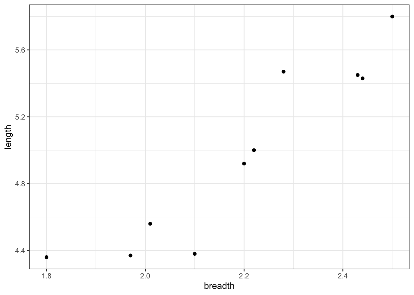
Figure 7.2: A small data set with the measurements of ten flint tools.
7.2.2 Implementing cross-validation in regression
Define \(D=\{(x_i,y_i),\, i=1,\ldots,10\}\) to be the full data set, with \(x_i\) and \(y_i\) the breadth and length, respectively, in mm, for the \(i^\text{th}\) tool. We’ll consider a simple linear regression model of the form \[Y_i = \beta_0 + \beta_1 x_i + \varepsilon_i,\] with \(\varepsilon_i \sim N(0,\sigma^2)\).
Given parameter estimates \(\hat{\beta}_0\) and \(\hat{\beta}_1\) and a tool breadth \(x\), we would predict the corresponding tool length as \(\hat{y}=\hat{\beta}_0+\hat{\beta}_1x\), and we can obtain a prediction interval using standard theory.
Linear models are well understood, and there are various diagnostics we can do to check goodness-of-fit, model assumptions and so on, so that we wouldn’t normally consider cross-validation methods. However, as the sample size is so small, it’s going to be harder to judge from the usual diagnostics whether we can really trust predictions from our model. Despite this, it would be interesting to get some idea how the model performs on ‘new’ observations. Further, we could apply the same ideas for more complex, ‘black-box’ regression models, where we don’t have the same diagnostic tools that we have for simple linear regression.
We’ll use cross-validation in a similar way as before, removing each observation in term and forming a prediction. To obtain this prediction, we will re-estimate the model parameters each time, and also compute a prediction interval in addition to an estimate \(\hat{y}_i\). The procedure is as follows.
For \(i=1,\ldots,10\):
- Remove the observation \((x_i,y_i)\) from the data set \(D\) to get a reduced data set \(D_{-i}\).
- Using \(D_{-i}\), compute least squares estimates of \(\beta_0\) and \(\beta_1\), and estimate \(\sigma^2\) with the corresponding residual sum of squares. Denote these estimates by \(\hat{\beta}_{0,i}\) and \(\hat{\beta}_{1,i}\), and \(\hat{\sigma}^2_i\) respectively.
- Estimate the \(i^\text{th}\) tool length using \[\hat{y}_i=\hat{\beta}_{0,i}+\hat{\beta}_{1,i}x_i,\] and obtain the corresponding (95%) prediction interval.
These estimates and intervals can then be compared with the original observations \(y_1,\ldots,y_{10}\).
In R, we’ll first set up an empty matrix to take the results:
In R, we implement this as:
flint_yhat <- matrix(NA, nrow = 10, ncol = 3)

for(i in 1:10){

  lmReduced <- lm(length ~ breadth, subset = -i, data = flint)
  flint_yhat[i, ] <- predict(lmReduced, flint[i, ], interval = "prediction")

}
Figure 7.3 displays the results of this cross-validation experiment. For each observed breadth, the true length is shown in red. The fitted regression line from the complete set of 10 observations is shown in grey. The cross-validation results are shown in black, both as a point estimate and an interval. Note that the predictions do not sit on the regression line because they are each obtained by removing that observation from the training data. We can see, however, that the cross-validation predictions are in most cases close to the full data prediction which tells us that no single observation is having a great effect on the predicted model coefficients.
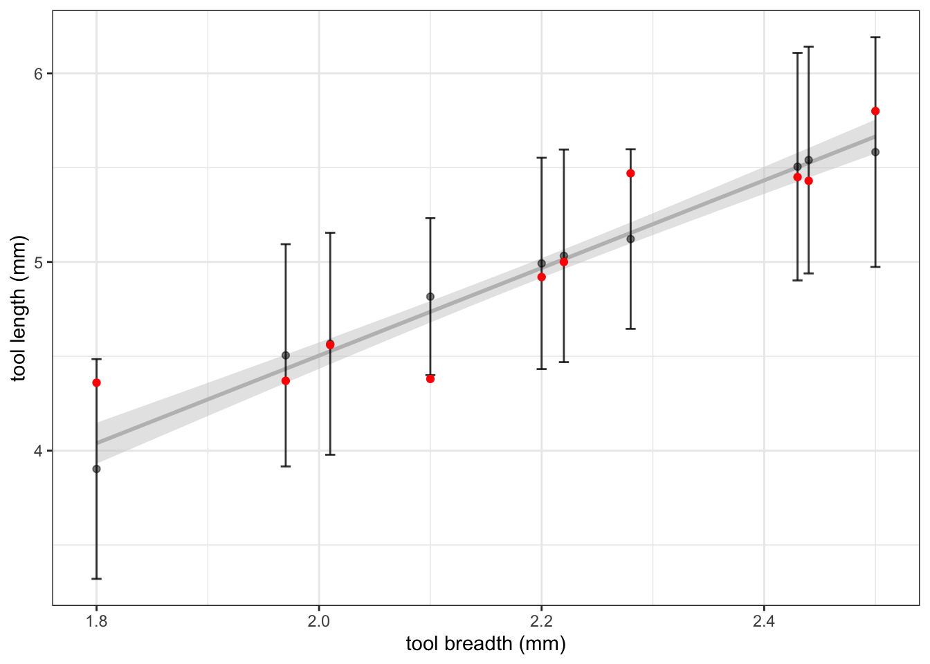
Figure 7.3: The results of cross-validation on the flint tools data. The observed data is shown in red. Predictions (black point) of the length, and intervals, are shown for each breadth measurement, obtained by removing that measurement from the training data. The regression line using all 10 observations is also included for comparison.
7.3 Parameter estimation with cross-validation
So far, we’ve used cross-validation to check how well a model (or algorithm) predicts observations. But we can also use it to estimate/choose parameters in our model/algorithm. We define a loss function \(L(\hat{y}_i, y_i)\) which gives a penalty for predicting a value \(\hat{y}_i\), using the reduced data set \(D_{-i}\), when the true value is \(y_i\). We could then choose our model parameters to minimise \[\sum_{i=1}^n L(\hat{y}_i, y_i).\]
7.3.1 Example: choosing the value \(K\) in KNN
Recall that in the KNN algorithm we have to decide how many ‘nearest neighbours’ \(K\) to look for. Note that in the penguin example earlier, we implemented \(K=1\). This parameter could be selected using cross-validation. An appropriate loss function would be \[L(\hat{y}_i, y_i) = \begin{cases} 0 & \text{for }\hat{y}_i= y_i;\\ 1 & \text{for }\hat{y}_i\neq y_i. \end{cases}\] This loss function would lead to us searching for the \(K\) that minimises the number of incorrect predictions.
We’ll try this for the Palmer penguins. We’ve already seen that the algorithm works about as well as we could hope for using \(K=1\) as there was only 7 incorrect predictions, so there’s not really any scope for improvement, but just for illustration, we’ll try a few different \(K\).
Rather than using a for loop, we’ll use the function knn.cv(), which implements cross-validation for us:
peng_yhat <- class::knn.cv(train = X, cl = y, k = 1)
peng_yhat10 <- class::knn.cv(train = X, cl = y, k = 10)
peng_yhat100 <- class::knn.cv(train = X, cl = y, k = 100)
The sum of the loss functions for these \(K\) are then 7, 6 and 20, respectively for \(k=1,10,100\). As we expected, there isn’t an argument for increasing the complexity of our classification algorithm here (as for \(K>1\) we have to identify the most common classification from a number of neighbours) because there isn’t much difference between \(K=1\) or 10, but the performance is markedly worse for \(K=100\).
7.3.2 Cross-validation as an alternative to maximum likelihood
For the KNN algorithm, there is no model; we couldn’t write down a likelihood function. Cross-validation is a natural way to choose \(K\): if we didn’t remove \(y_i\) before predicting it, the nearest neighbour to the \(i\)-th observation would be itself, and we’d always get 100% prediction accuracy with \(K=1\) (assuming the independent variables are all distinct).
When we do have a model, cross-validation could be used as an alternative way to estimate parameters; there are advantages and disadvantages. If we only care about getting good point predictions for new observations \(y\), cross-validation (with a suitable loss function) will attempt to get small prediction errors, regardless of whether the model assumptions are valid.
If we also care about quantifying uncertainty in our predictions, we could try to design a suitable loss function, but maximum likelihood may be preferable. With maximum likelihood, within our chosen model, we’re trying to find the parameters that can ‘best’ describe the distribution of the data, and this will help us with our uncertainty quantification.
As we’ll see later, there is a relationship between cross-validation and AIC, so cross-validation may be useful in situations where we want to penalise for model complexity.
7.4 Computational short-cuts
If we need to repeatedly do cross-validation, for example if we’re using it to estimate parameters, then the method can get computationally expensive. For example, if we have \(n\) observations, and we want to try \(d\) different parameter values to find the ‘best’ choice, we would have to fit the model \(n\times d\) times.
For linear models, it turns out that we don’t actually need to refit the model each time with a reduced data set: we can compute everything we need from a single model fit to all the data. There are similar results for some other types of model, so we need to be alert to this possibility, as it may speed up the computation.
For a linear model, given the full data set \(D\), define as follows:
- \(\hat{\beta}\): the least squares estimator of \(\beta\);
- \(X\): the design matrix;
- \(H\): the ‘hat matrix’ given by \(X(X^TX)^{-1}X^T\)
- \(f(x_j)^T\): the \(j^\text{th}\) row of the design matrix \(X\);
- \(r_j\): the \(j^\text{th}\) residual, \(r_j=y_j-f(x_j)^T\hat{\beta}\).
Now, when the \(i^\text{th}\) observation is removed from the data set \(D\), denote the corresponding least squares estimate by \(\hat{\beta}_{(i)}\) and define \[\begin{equation} r_{(i)} = y_i - f(x_i)^T\hat{\beta}_{(i)}, \tag{7.1} \end{equation}\] which is the difference between the \(i^\text{th}\) observed dependent variable and its estimate obtained when this observation is removed from the data \(D\). Note that \(r_{(i)}\) is sometimes referred to as the \(i^\text{th}\) deletion residual, and is not equal to \(r_i\) because the least squares estimators are different (one is based on the full dataset and the other is from the reduced data).
Earlier we used a for loop to compute \(\hat{\beta}_{(i)}\) and \(f(x_i)^T\hat{\beta}_{(i)}\) for \(i=1,\ldots,n\), removing each point in turn, refitting the model, and calculating the least squares estimate. But it isn’t necessary: it can be shown that \[\begin{equation} r_{(i)} = \frac{r_i}{1-h_{ii}}, \tag{7.2} \end{equation}\] and \[\begin{equation} \hat{\beta}_{(i)} = \hat{\beta} - (X^TX)^{-1}x_ir_{(i)}, \tag{7.3} \end{equation}\] where \(h_{ii}\) is the \(i^\text{th}\) diagonal element of the hat matrix \(H\). Proofs are given at the end of this chapter for reference, but you will not be assessed on these results or the proofs in this module.
In summary, we do not need to implement a for loop like earlier, refitting the model for each removed location. Instead, we only fit the model once to the full data-set, and then calculate each deletion residual based on Equation (7.2).
7.4.1 Example: Returning to the flint data
Let’s check this short cut in R on a data-set. First, we’ll fit the flint model using all the data, and obtain \(X\) and \(H\):
lmFull <- lm(length ~ breadth, data = flint)
X <- model.matrix(lmFull)
H <- X %*% solve(t(X) %*% X, t(X))
Then we’ll calculate the deletion residuals using the relationship in Equation (7.2):
(deletionResiduals <- lmFull$residuals/(1 - diag(H)))## 1 2 3 4 5 6
## -0.13517895 -0.11047994 -0.03252041 -0.43621461 -0.05516638 0.21738803
## 7 8 9 10
## 0.45743603 0.34848697 -0.07227648 -0.00645657We’ll check these are the same as the deletion residuals that are calculated via Equation (7.1) using the results from our earlier approach of using a for loop and repeatedly fitting the linear model on the reduced data:
flint$length - flint_yhat[ ,1]## [1] -0.13517895 -0.11047994 -0.03252041 -0.43621461 -0.05516638 0.21738803
## [7] 0.45743603 0.34848697 -0.07227648 -0.00645657They are equal!
We’ll also refit the model with the first observation removed to obtain \(\hat{\beta}_{(1)}\), and check we get the same as via Equation (7.3):
lmReduced <- lm(length~breadth, subset = -1, data = flint)
lmReduced$coefficients
## (Intercept) breadth
## 0.2820335 2.1437286lmFull$coefficients -
solve(t(X) %*%X, t(X[1, , drop = FALSE ])) * deletionResiduals[1]## 1
## (Intercept) 0.2820335
## breadth 2.1437286Again, these are equal!
7.5 Relationship with AIC
Stone (1977) established a relationship between cross-validation and Akaike’s Information Criterion (AIC). Recall that AIC is defined as \[-2 l(\hat{\theta}; y) + 2p,\] where \(l(\hat{\theta}; y)\) is the maximised log-likelihood function, and \(p\) is the number of parameters in the model. We can use AIC to compare models, with a lower AIC value indicating a better model fit, after penalising for the model complexity (number of parameters).
Now define a goodness-of-fit measure based on cross-validation as \[CV:= -2\sum_{i=1}^n \log \pi(y_i|x_i, D_{-i}, \hat{\theta}_{(i)})\] where \(\hat{\theta}_{(i)}\) is the maximum likelihood estimate of the parameters given the reduced data set \(D_{-i}\), and \(\pi()\) is the predictive density function of the model. For example, in our simple linear regression model, we would have \[y_i \ | \ x_i, D_{-i}, \hat{\theta}_{(i)} \sim N((1,\, x_i)\hat{\beta}_{(i)}, \ \hat{\sigma}^2_{(i)}),\] so that \[\pi(y_i|x_i, D_{-i}, \hat{\theta}_{(i)}) = \frac{1}{\sqrt{2\pi\hat{\sigma}^2_{(i), MLE}}}\exp\left(-\frac{1}{2\pi\hat{\sigma}^2_{(i), MLE}}(y_i - (1,\, x_i)\hat{\beta}_{(i)})^2\right),\] where \(\hat{\sigma}_{(i), MLE}\) is the maximum likelihood estimator of \(\sigma^2\), given the reduced data set \(D_{-i}\). Stone then shows that asymptotically, \(CV\) is equivalent to AIC. Intuitively, as the sample size tends to infinity, the maximised log-likelihood would dominate the penalty term \(2p\), and we would expect \(\hat{\theta}_{(i)}\) to be similar to \(\hat{\theta}\), so that both AIC and \(CV\) are just reporting the maximised log-likelihood. But this does suggest that cross-validation does have the effect of penalising for model complexity, in a similar way to AIC.
7.5.1 Example: The cars data
We’ll use the cars data, one of R’s in-built datasets, and consider a simple linear regression model to predict stopping distance (dist) given the initial travelling speed (speed) for some (very old!) cars. There are 50 observations in this data set.
We’ll first fit the model to all the data:
lmFull <- lm(dist ~ speed, data = cars)This gives the AIC as 419.156863 and minus twice the maximised log likelihood as 413.156863.
Now we’ll compute \(CV\). We’ll go back to using a for loop, to make the code a bit more readable:
X <- model.matrix(lmFull)
n <- nrow(X)
y <- cars$dist
logPredictiveDensity <- rep(NA, n )

for(i in 1:n) {

  lmCV <- lm(dist ~ speed, subset = -i, data = cars)
  # Need the MLE of sigma. We've got n-1 observations so this is RSS/(n-1)
  #sigmaMLE <- sqrt(sum(lmCV$residuals^2) / (n - 1))
  logPredictiveDensity[i] <- dnorm(y[i],
                                   sum(X[i, ]*lmCV$coefficients),
                                   sigma(lmCV),
                                   log = TRUE)
}

-2 * sum(logPredictiveDensity)
## [1] 421.028This is close to the value obtained by AIC, and closer than when compared with minus twice the maximised log likelihood so it does appear that \(CV\) is penalising for the number of parameters.
7.6 (Non-examinable) Proof of the computational short cut
We outline how to derive the expressions for \(r_{(i)}\) and \(\hat{\beta}_{(i)}\) in Equations (7.2) and (7.3).
7.6.1 Helpful results we will use
There are two results that help us here (and then it’s just fairly straightforward algebra - we won’t give all the steps here). Recall that \(f(x_i)^T\) is the \(i\)-th row of the design matrix \(X\).
The first result is that \[ X^TX = \sum_{i=1}^n f(x_i)f(x_i)^T, \] so we can write \[\begin{equation} X^T_{(i)}X_{(i)} = X^TX - f(x_i)f(x_i)^T, \tag{7.4} \end{equation}\] where \(X_{(i)}\) is the design matrix with the \(i\)-th row (observation) removed. We will use this result multiple times in the following to relate the full dataset to the reduced dataset.
The second result is the Woodbury identity for matrix inversion: \[ (A+UCV^T)^{-1} = A^{-1} - A^{-1}U(C^{-1} + V^TA^{-1}U)^{-1}VA^{-1}, \] for matrices of the appropriate sizes (with \(A\) and \(C\) invertible). To relate this to our scenario, we equate
- \(X^TX\) with \(A\),
- \(U\) with \(-f(x_i)\),
- \(V\) with \(f(x_i)\),
and set \(C\) to be the (\(1\times 1\)) identity matrix. After a little algebra we have \[\begin{equation} (X^T_{(i)}X_{(i)})^{-1} = (X^TX)^{-1} + \frac{(X^TX)^{-1}f(x_i)f(x_i)^T(X^TX)^{-1}}{1 - h_{ii}}, \tag{7.5} \end{equation}\] where \(h_{ii}\) is the \(i\)-th diagonal element of \(X(X^TX)^{-1}X^T\).
7.6.2 Relate the estimated coefficients of full and reduced models
Next, we relate \(\hat{\beta}\) with \(\hat{\beta}_{(i)}\).
Define \(y_{(i)}\) to be the vector of all observations, with \(y_i\) removed, so that the estimated coefficients when the \(i^\text{th}\) observation is removed is \[\begin{equation} \hat{\beta}_{(i)} = (X^T_{(i)}X_{(i)})^{-1}X^T_{(i)}y_{(i)}. \tag{7.6} \end{equation}\] Equation (7.4) also tells us that \[\begin{equation} X^T_{(i)}y_{(i)} = X^Ty - y_i f(x_i). \tag{7.7} \end{equation}\] Substituting Equations (7.5) and (7.7) into Equation (7.6) gives \[ \hat{\beta}_{(i)} = (X^TX)^{-1}(X^Ty - y_i f(x_i)) + \frac{(X^TX)^{-1}f(x_i)f(x_i)^T(X^TX)^{-1}(X^Ty - y_i f(x_i)) }{1 - h_{ii}}. \] which, after some algebra, becomes \[\begin{equation} \hat{\beta}_{(i)} = \hat{\beta} - (X^TX)^{-1}f(x_i)\frac{r_i}{1 - h_{ii}}. \tag{7.8} \end{equation}\]
7.6.3 Relating the residuals
We have that the deletion residual is \[ r_{(i)} = y_i - f(x_i)^T\hat{\beta}_{(i)}, \] and after substituting in Equation (7.8) for \(\hat{\beta}_{(i)}\), we get \[ r_{(i)} = \frac{r_i}{1-h_{ii}}. \]